You can define rebar in shell, membrane, continuum, and beam elements as an
element property.
However, this method is more cumbersome than the method described
in Defining Reinforcement and does not allow
visualization of the rebar and rebar results in Abaqus/CAE.
The preferred method for defining rebar in shell, membrane, and beam elements is
defining rebar layers (rebar lines for beam elements) of reinforcement as part of the element
section definition (documented in Defining Reinforcement). The preferred method
for defining rebar in solids is embedding reinforced surface or membrane elements in “host”
solid elements as described in Embedded Elements.
Element-based
rebars:
are used to define uniaxial reinforcement in solid, membrane, shell, and beam elements;
can be defined as individual reinforcing bars in solid elements;
can be defined as layers of uniformly spaced reinforcing bars in shell, membrane, and solid
elements (such layers are treated as a smeared layer with a constant thickness equal to the
area of each reinforcing bar divided by the reinforcing bar spacing);
can be used with coupled temperature-displacement elements but do not contribute to the
thermal conductivity and specific heat;
can be used with coupled thermal-electrical-structural elements but do not contribute to
the electrical conductivity, thermal conductivity and specific heat;
do not contribute to the mass of the model in Abaqus/Standard;
cannot be used in elements intended for heat transfer or mass diffusion analysis;
cannot be used with triangular shell and membrane elements or with triangular, triangular
prism, and tetrahedral solid elements; and
have material properties that are distinct from those of the underlying element.
You must assign a name to the rebar set. This name can be used in defining rebar prestress
and output requests. Each layer of rebar must be assigned a separate name in a particular
element or element set.
Defining Rebars in Three-Dimensional Shell and Membrane Elements
Both isoparametric and skew rebars can be defined in three-dimensional shell and membrane
elements. Rebars cannot be used with triangular shells or membranes.
If triangular-shaped shells or membranes are needed, collapsed quadrilateral shells or
membranes can be used. The resulting rebar directions will depend on the type of rebar
(isoparametric or skew) used. The rebar must be defined carefully since the element is
distorted. This technique should be used only in regions of the mesh where results are not
critical and stress gradients are not high.
The stiffness calculations for the rebars use the same integration points as the
calculations for the underlying shell or membrane elements. See About Shell Elements and Membrane Elements for more
information about shell and membrane elements.
Defining Isoparametric Rebars in Three-Dimensional Shell and Membrane Elements
Isoparametric rebars are aligned along the mapping of constant isoparametric lines in the
element (see Figure 1).
Figure 1. “Isoparametric” rebar in an undistorted three-dimensional shell or membrane
element.
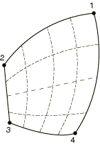
If opposite edges of the element containing the rebar are not parallel, the rebar
directions will be different at each of the integration points within an element (see
Figure 2).
Figure 2. “Isoparametric” rebar directions in a distorted three-dimensional shell or membrane
element (dashed lines indicate rebar directions).
The spacing of the rebar will be fixed in physical space. The spacing,
s, and the area of the rebar, A, are used to
determine the thickness of the equivalent smeared layer, . If the edges of the element containing the rebar are not parallel, the
number of actual rebar with this spacing passing through one edge will be different than
the number passing through the opposite edge (opposite in isoparametric space).
You specify the elements that contain the rebars; the cross-sectional area,
A, of each rebar; the rebar spacing in the plane of the shell,
s; and the edge number to which the rebars are parallel when plotted
in isoparametric space (see Figure 1). In addition, for shell elements you specify the position of the rebars in the shell
thickness direction measured from the midsurface of the shell (positive in the direction
of the positive normal to the shell). If the shell's thickness is defined by nodal
thicknesses (Nodal Thicknesses), this distance is scaled by the
ratio of the thickness defined by the nodal thickness to the thickness defined by the
section definition. If the shell's thickness is defined with a distribution (Distribution Definition), this distance is scaled by the ratio of the
element thickness defined by the distribution to the default thickness. If the shell has a
composite section whose layer thicknesses are defined with distributions (Distribution Definition), this distance is scaled by the ratio of the
sum of the element layer thicknesses defined by the distributions to the sum of the
default layer thicknesses.
Input File Usage
Use the following option to define isoparametric rebars in three-dimensional shell
elements:
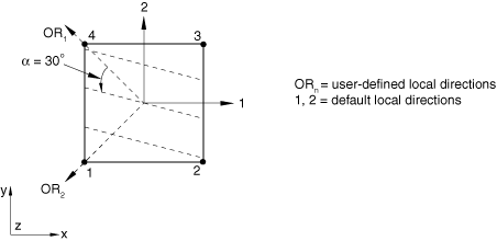
Defining Skew Rebars in Three-Dimensional Shell and Membrane Elements
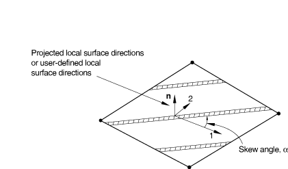
Skew rebars need not be similar to an element edge; they can lie at any prescribed angle
from the local 1-axis. The direction of the rebars must be defined in one of two ways, as
indicated in Figure 3:
Figure 3. “Skew” rebar in a three-dimensional shell or membrane.
The rebars can be defined relative to the default projected local coordinate system
(see Conventions).
The rebars can be defined relative to a user-defined local coordinate system (see
Orientations).
The orientation definition that can optionally be associated with a shell or membrane
section definition has no influence on the rebar angular orientation definitions. If the
shell or membrane is curved in space, the local 1-direction will vary across the element
and the skew rebar will also vary accordingly.
For shell elements the definition of a local coordinate system using distributions (Distribution Definition) has no influence on the rebar angular
orientation definitions.
If the rebar cross-sectional area is A, the rebar spacing,
s, should be given so that the thickness of the equivalent “smeared”
layer of reinforcing is .
Defining Skew Rebars Relative to the Default Projected Local Coordinate
System
To define skew rebars relative to the default projected local coordinate system, you
specify the elements that contain the rebars; the cross-sectional area,
A, of each rebar; the rebar spacing in the plane of the shell,
s; the position of the rebars in the thickness direction (for shell
elements only), measured from the midsurface of the shell (positive in the direction of
the positive normal to the shell); and the angle , in degrees, between the default local 1-direction and the rebars. See
Conventions for a definition of the default projected local
directions on a surface in space. If the shell's thickness is defined by nodal
thicknesses (Nodal Thicknesses), the rebar position in the
thickness direction will be scaled by the ratio of the thickness defined by the nodal
thickness to the thickness defined by the section definition. If the shell's thickness
is defined with a distribution (Distribution Definition), the
rebar position in the thickness direction is scaled by the ratio of the element
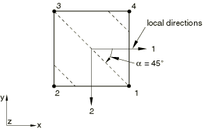
thickness defined by the distribution to the default thickness. A positive angle defines a rotation from local direction 1 to local direction 2 around
the element's normal direction. For example, in a membrane the following data would
result in the rebar definition shown in Figure 4: A=0.05, s=0.1, and =45.
Figure 4. Skew rebar defined relative to default local coordinate directions.
When a user-defined local orientation definition is not used to define the angular
orientation of the rebar and the normal to the shell is nearly parallel to the global
1-axis, the local 1-axis may change significantly within an element or from one element
to the next (see Conventions).
Input File Usage
Use the following option to define skew rebars relative to the default projected
local coordinate system in three-dimensional shell elements:
Defining Skew Rebars Relative to a User-Defined Local Coordinate System
To define skew rebars relative to a user-defined local coordinate system, you specify
the elements that contain the rebars; the cross-sectional area, A,
of each rebar; the rebar spacing in the plane, s; the position of
the rebars in the thickness direction (for shell elements only), measured from the
midsurface of the shell (positive in the direction of the positive normal to the shell);
and the angle, , in degrees, between the user-defined 1-direction and the rebars. See
Orientations for a description of how the local coordinate
system is calculated from the user-defined directions for definition of rebar in shells
and membranes. A positive angle defines a rotation from local direction 1 to local direction 2 around
the user-defined normal direction. For example, in a shell the following data would
result in the skew rebar definition shown in Figure 5: A=0.01; s=0.1; distance of rebar from the
shell midsurface=0.0; =30.; and the rebar definition refers to a local rectangular
orientation defined to have its X-axis go through the point
(−0.7071, 0.7071, 0.0), its X–Y plane include
the point (−0.7071, −0.7071, 0.0), and an additional rotation of 0.0 degrees about the
3-direction.
Figure 5. Skew rebar defined relative to user-defined local coordinate directions.
Input File Usage
Use the following option to define skew rebars relative to a user-defined local
coordinate system in three-dimensional shell elements:
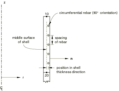
Defining Rebars in Axisymmetric Shell and Membrane Elements
Rebars in an axisymmetric membrane must lie in the membrane reference surface, whereas
rebars in an axisymmetric shell can lie in the shell reference surface or can be offset from
the midsurface. Rebars in axisymmetric shells and membranes can be defined to have any
orientation with respect to the r–z plane. See
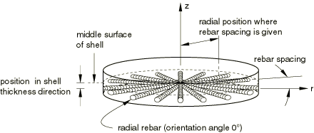
Figure 6 for an example of circumferential rebars and Figure 7 for an example of radial rebars in axisymmetric shells.
Figure 6. Example of circumferential rebars in axisymmetric shell elements. Figure 7. Example of radial rebars in axisymmetric shell elements.
You specify the cross-sectional area, A, of each rebar; the rebar
spacing, s; for shell elements the position of the rebars in the shell
thickness direction, measured from the midsurface of the shell (positive in the direction of
the positive normal to the shell); the angular orientation with respect to the
r–z plane, , measured in degrees; and the radial position at which the rebar spacing
is measured. The angular orientation is measured positive about the positive normal to the
shell or membrane element. If the shell's thickness is defined by nodal thicknesses (Nodal Thicknesses), the distance from the midsurface will be scaled by
the ratio of the thickness defined by the nodal thickness to the thickness defined by the
section definition. If the shell's thickness is defined with a distribution (Distribution Definition) the distance from the midsurface will be
scaled by the ratio of the element thickness defined by the distribution to the default
thickness.
If an orientation angle other than 0 or 90° is specified for rebar in an axisymmetric shell
or membrane without twist, Abaqus assumes that the rebars are balanced (i.e., half the rebar lie at the specified angle and the other half at an angle of ) and internal calculations are handled accordingly. See Rebar modeling in two dimensions for details. If
the symmetric model generation capability (Symmetric Model Generation) is used to create
a three-dimensional model from an axisymmetric shell or membrane model, only balanced rebars
will be translated appropriately. The definition of balanced rebars in the axisymmetric
model will result in balanced rebars in the three-dimensional model; such a translation with
unbalanced rebars is not available. Unbalanced rebars in generalized axisymmetric membranes
with twist will be translated properly.
If the radial position for the rebar spacing is given, the total cross-sectional area of
rebar will remain constant as the radial position changes; this behavior corresponds to the
number of rebar in the circumferential direction remaining constant and implies that the
thickness of the smeared layer of rebar decreases and that the spacing of the rebars
increases as r increases (see Figure 7). If the radial position for the rebar spacing is omitted (or is set to zero), Abaqus assumes that the spacing of the rebar remains constant; the thickness of the
corresponding smeared layer is held fixed such that .
Input File Usage
Use the following option to define rebars in an axisymmetric shell element:
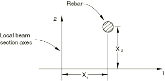
You can use element-based rebar to model discrete rebar in beam elements in Abaqus/Standard and Abaqus/Explicit. You specify the elements that contain the rebar, the
cross-sectional area of each rebar, and the location of each rebar with respect to the local
beam section axis (see Figure 8).
You must assign each individual rebar a separate name in a particular element or element
set.
Figure 8. Rebar location in a beam section.
Input File Usage
Use the following option to define rebar in beam elements:
Two- or three-dimensional continuum (solid) elements can contain rebars; rebars cannot be
defined in triangular, prism, tetrahedral, or infinite elements. If triangular or
wedge-shaped elements are needed, collapsed quadrilateral or brick elements can be used. Be
careful when collapsing elements that contain rebar. It is important to check that the
location and orientation of the rebar are correct.
Rebars are defined as single bars or in layers. In the latter case the layer is a surface
in each element; you provide the rebar orientation in the surface.
Defining Layers of Rebars in Planar and Axisymmetric Continuum Elements
By default, the rebars form a layer that lies in a surface that is at right angles to the
plane of the model. You define the line where this rebar surface intersects the plane of
the model, as described below.
The orientation of the rebars within the rebar surface is defined by giving an angle, in
degrees, between the line of intersection in the plane of the model and the rebars. This
angle is measured in physical three-dimensional space, not in isoparametric space. See
Rebar modeling in two dimensions for details. The
positive direction along the line of intersection is from the lower to the higher numbered
element edge that is intersected, and a positive angle indicates rebars oriented down into
the plane of the model (where the plane is parallel to the z-axis in
plane strain analysis or the -axis for axisymmetric analysis), as shown in Figure 9.
Figure 9. Orientation of rebars in plane and axisymmetric solid elements.
If an orientation angle other than 0 or 90° is specified for rebar in an axisymmetric
element without twist, it is assumed that the rebar in the element are balanced (i.e.,
half the rebar lie at the specified angle and the other half at the angle ).
Defining Isoparametric Rebars
For isoparametric rebars the intersection of the rebar layer with the plane of the
model will lie along the mapping of a constant isoparametric line in the element. You
specify the elements that contain the rebars; the cross-sectional area,
A, of each rebar; the rebar spacing, s; the
rebar orientation, (as described above); the fractional distance
from the edge, f (the ratio of the
distance between the edge and the rebar to the distance across the element); and the
edge number from which the rebars are defined. In addition, for axisymmetric elements
you specify the radial position at which the rebar spacing is measured.
If the radial position for the rebar spacing is given for rebar in axisymmetric
elements, the total cross-sectional area of rebar will remain constant as the radial
position changes; this behavior corresponds to the number of rebar remaining constant as
r increases; that is, the thickness of the smeared layer of rebar
decreases as r increases. If the radial position for the rebar
spacing is omitted (or is set to zero), Abaqus assumes that the spacing of the rebar remains constant; the thickness of the
corresponding smeared layer is held fixed such that .
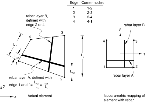
Figure 10 shows an example of isoparametric rebar.
Figure 10. Isoparametric rebar layer definition in solid elements.
In the isoparametric mapping of the element, the line of rebars is parallel to one of
the edges of the element. In this figure the line for rebar layer A
can be defined using edges 1 or 3 and rebar layer B can be defined
by edges 2 or 4. The fractional distance from edge 1 for rebar layer
A is the ratio ; alternatively, layer A can be defined from edge
3, so that .
Input File Usage
Use the following option to define layers of isoparametric rebars in planar and
axisymmetric continuum elements:
For skew rebars the intersection of the rebar layer with the plane of the model can
intersect any two edges of an element. You specify the elements that contain the rebars;
the cross-sectional area, A, of each rebar; the rebar spacing,
s; and the rebar orientation, (as described above). In addition, for axisymmetric elements you
specify the radial position at which the rebar spacing is measured. You also specify the
fractional distance along the element edge, from the first
node of the edge (as listed in Figure 11) to where the rebar layer intersects the edge, for all edges. Only the two values
corresponding to the two edges that the rebar intersects can be nonzero.
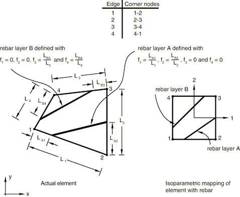
Figure 11. Skew rebar layer definition in solid elements.
Figure 11 shows an example of skew rebar. In the isoparametric mapping of the element, the line
of rebars intersects two of the element edges. The intersection points are located by
defining a fractional distance along each intersected edge. In this figure rebar layer
A is defined by the ratio along edge 1 and the ratio along edge 2. Rebar layer B is defined by the
ratio along edge 3 and the ratio along edge 4.
Defining skew rebars in continuum elements can increase the run time for an Abaqus/Explicit analysis significantly. The element's stable time increment will, in most cases, be
determined by the stable time increment of the rebar, which is proportional to the rebar
length. The rebar length is determined by factors including the rebar surface position
in the element, the rebar spacing, the rebar area, and the rebar orientation within the
rebar surface. If a skew rebar in a continuum element is defined such that it intersects
two adjacent element edges, the resulting rebar length could be considerably less than
the average element edge length, thus resulting in a very small element stable time
increment.
Input File Usage
Use the following option to define layers of skew rebars in planar and
axisymmetric continuum elements:
Defining Single Rebars in Two-Dimensional Axisymmetric and Generalized Plane Strain
Continuum Elements
You can define single rebars in axisymmetric and generalized plane strain continuum
elements. In this case the rebar is assumed to be at right angles with the plane of the
model—in the thickness direction for generalized plane strain elements or the hoop
direction for axisymmetric elements.
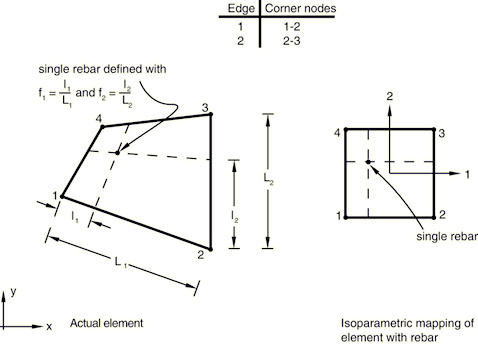
The intersection of the rebar with the plane of the model is defined by the fractional
distances along edges 1 and 2 of the intersections of constant isoparametric lines that
pass through the rebar location (see Figure 12). The fractional distances are measured from the first edge node listed in Figure 12.
Figure 12. Single rebar in a solid element.
You specify the elements that contain the rebars; the cross-sectional area,
A, of each rebar; and the fractional distances locating the rebar's
position in the element, and .
Input File Usage
Use the following option to define single rebars in axisymmetric and generalized
plane strain continuum elements:
Defining Layers of Rebars in Three-Dimensional Continuum Elements
By default, the rebars in three-dimensional continuum elements are defined as layers
lying in surfaces. The surfaces are most easily defined with respect to the isoparametric
mapped cube of the element. Therefore, you must consider how the rebar will be defined
before generating the mesh; if the rebar surfaces are not taken into account in designing
the mesh, the rebar definition can be very inefficient.
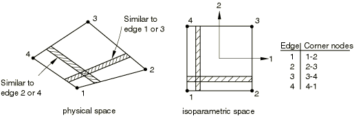
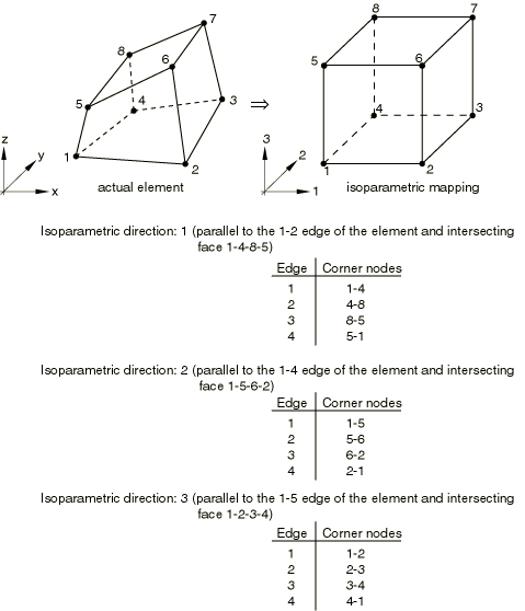
In the isoparametric mapped cube the rebar surface always has two edges (opposite to one
another) that are parallel to an isoparametric direction. The isoparametric directions are
defined in Figure 13. You specify this isoparametric direction (1, 2, or 3).
Figure 13. Isoparametric direction and edge definitions for three-dimensional
elements.
A particular face of the element, which is perpendicular to this isoparametric direction
in the isoparametric mapped cube, is used to define the position of the other two edges of
the surface; the faces are defined in Figure 13, where the edges of the faces are also defined.
If isoparametric rebars are defined, the two edges of the rebar surface that are not
parallel to the user-specified isoparametric direction will be parallel to one of the
other two isoparametric directions; in the isoparametric-mapped cube one isoparametric
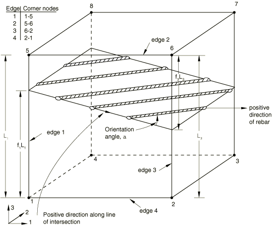
coordinate is constant on the rebar surface. Figure 14 illustrates this concept with an element containing two layers of isoparametric rebars.
Figure 14. Element with two layers of isoparametric rebar.
The position of each surface is given by the fractional distance f
from an edge of the face defined in Figure 13 for the isoparametric direction chosen; you must specify the edge from which the
fractional distance is measured.
If skew rebars are defined, the two edges of the rebar surface, which are not parallel to
the user-specified isoparametric direction, are generally not parallel to one of the other
isoparametric directions. The positions of these two edges of the rebar surface are
specified by the intersection of the rebar surface with edges of the intersecting face,
defined in Figure 13, for the isoparametric direction chosen; the intersections are given by the fractional
distance f along each edge of the face. (Note that the fractional
distance is along the edge for skew rebars; for isoparametric
rebars the fractional distances are measured from an edge.)
The fractional distance along an edge is measured from the first node of the edge. All
four fractional distances must be given, but only two can be nonzero.
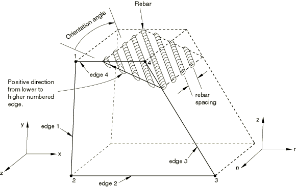
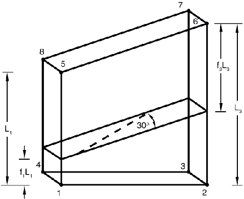
The orientation angle, , of the rebars within the rebar layer is defined in the
isoparametric-mapped cube; it is measured in degrees and is the angle between the line of
intersection of the rebar surface with the face for the isoparametric direction chosen and
the rebar. The positive direction of the line of intersection is from the lower numbered
edge to the higher numbered edge; the positive direction for the rebars points into the
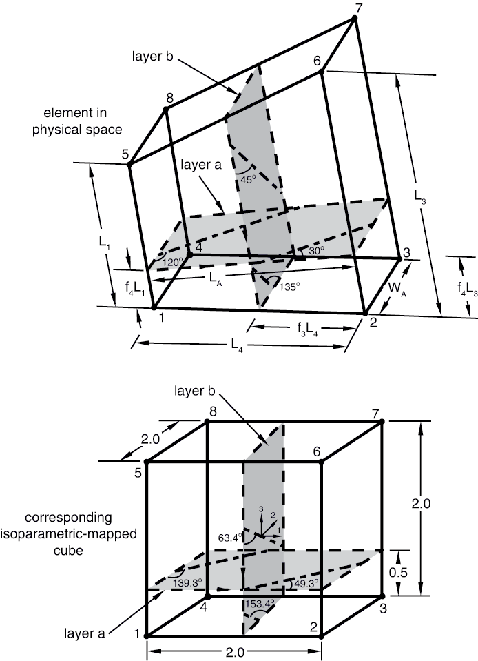
elements. An example is shown in Figure 15. The orientation angle is defined in the rebar layer in the isoparametric-mapped cube;
therefore, the definition is the same for isoparametric and skew rebar.
Figure 15. Orientation example for three-dimensional skew rebar modeling, isoparametric
direction 2. Shown in the mapped isoparametric element.
If the rebar layer is not flat in physical space, the orientation angle at each
integration point may be different. Since it is possible to define only one orientation
angle per element, an average value orientation angle for the element must be used; for
reasonable meshes this approximation should not affect the results significantly.
Defining Isoparametric Rebars
You specify the elements that contain the rebars; the cross-sectional area,
A, of each rebar; the rebar spacing, s; the
rebar orientation, (as described above); the fractional distance, f,
from the edge; the number of the edge from which the fractional distance is measured;
and the isoparametric direction of the rebar surface.
Input File Usage
Use the following option to define layers of isoparametric rebars in
three-dimensional continuum elements:
Rebar layers A and B are defined using
isoparametric direction 2. From Figure 13 the position of the layers must be given with respect to the face with nodes 1-5-6-2.
The fractional distance defining the position of intersection of layer
A with this face can be measured from edge 4 (edge with nodes 2–1)
along edge 3 (edge with nodes 6–2), as shown in Figure 14. For layer A, . It could also be given from edge 2 (edge with nodes 5–6), so that .
The orientation of rebar for layer A in physical space is defined
by an angle, , equal to 30° for layer A. This angle must be
transformed into the corresponding angle in the isoparametric-mapped cube. This
transformation can be done as follows: consider a single rebar that intersects the
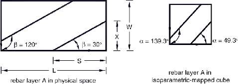
intersecting line (described above) and an adjacent edge (see Figure 16).
Figure 16. Example defining isoparametric rebar.
From the figure . The length of the rebar layer along the intersecting line is
L, and the length of the opposite edge is W.
Consider the same rebar in the rebar layer in the isoparametric-mapped cube. The
orientation angle, , is given by , where and . (The 2 is included because the isoparametric-mapped cube is a 2 × 2 ×
2 cube.) This expression can be simplified to give
For layer A, , , , and , where is the orientation angle that must be specified.
The fractional distance defining the position of the intersection of layer
B with this face can be measured from edge 3 (edge with nodes 6–2); . It could also be measured from edge 1 (edge with nodes 1–5), such
that . The orientation angle for layer B in the rebar
layer is 45°. In the isoparametric-mapped cube , , , and .
Since an isoparametric rebar layer always lies in two of the isoparametric directions,
an alternative but equivalent definition can be given. For example, layer
A also lies in isoparametric direction 1, with the intersecting
face having nodes 1-4-8-5. The fractional distance for layer A,
measured from edge 1 (edge with nodes 1–4), is . The positive sense of the line of intersection is from edge 2 (edge
with nodes 4–8) to edge 4 (edge with nodes 5–1); therefore, , , , and .
Layer B also lies in isoparametric direction 3, with the
intersecting face having nodes 1-2-3-4. The fractional distance for layer
B, measured from edge 2 (edge with nodes 2–3), is . The positive sense of the intersecting line is from edge 1 (edge with
nodes 1–2) to edge 3 (edge with nodes 3–4); therefore, the orientation angle of the
rebar in physical space is , , , and in the isoparametric-mapped cube .
Defining Skew Rebars
You specify the elements that contain the rebars; the cross-sectional area,
A, of each rebar; the rebar spacing, s; the
rebar orientation, (as described above); and the isoparametric direction. In addition,
you specify the fractional distance
falong the element edge for each edge
of the intersecting face defined in Figure 13. Only the values corresponding to the two edges that the rebar intersects can be
nonzero.
Input File Usage
Use the following option to define layers of skew rebars in three-dimensional
continuum elements:
The rebar layer is defined using isoparametric direction 2. The intersecting face is
defined in Figure 13 and has nodes 1-5-6-2. The position of the rebar layer is given by its intersection
with the edges of this face; the fractional distances, and , are shown in Figure 17. The orientation angle of the rebar in physical space is 30°. Following the same procedure
for calculating as was described for isoparametric rebar, , , and the orientation angle in the isoparametric-mapped cube is 55.28°.
Defining Single Rebars in Three-Dimensional Continuum Elements
You can define single rebars in three-dimensional continuum elements; in this case the
rebar is assumed to be placed along one of the element's isoparametric directions. The
rebar is then located by its intersection with the intersecting face (defined in Figure 13). The intersections of constant isoparametric lines with edges 1 and 2 of the
intersecting face are given by fractional distances along edges 1 and 2, measured from the
first node of each edge, as shown in Figure 12.
You specify the elements that contain the rebars; the cross-sectional area,
A, of each rebar; the fractional distances locating the rebar's
position in the element, and ; and the isoparametric direction. Give the fractional distances with
respect to edge 1 and edge 2 for the isoparametric direction chosen, as defined in Figure 13.
Input File Usage
Use the following option to define single rebars in three-dimensional continuum
elements:
The material properties of the rebars are distinct from those of the underlying element and
are defined by a separate material definition (Material Data Definition). You must
associate each rebar definition with a set of material properties.
The following material behavior cannot be used in Abaqus/Standard to define rebar materials:
In Abaqus/Standard density is ignored for the rebar material properties. Hence, the mass of the rebar is
neglected in eigenvalue extraction and implicit dynamic procedures and for gravity,
centrifugal, and rotary acceleration distributed loads.
Input File Usage
Use the following option to associate a material definition with a rebar
definition:
Initial conditions (Initial Conditions) can be used to
define rebar prestress or solution-dependent values for rebars.
Defining Prestress in Rebar
For structures in which reinforcing is defined (such as reinforced concrete structures),
you can use initial conditions to define the prestress in the rebars.
In such cases in Abaqus/Standard the structure must be brought to a state of equilibrium before it is actively loaded by
means of an initial static analysis step (Static Stress Analysis) with no
external loads applied (or, perhaps, with the “dead” loads only)—see Defining Initial Stresses.
Input File Usage
INITIAL CONDITIONS, TYPE=STRESS, REBARelement number or element set name, rebar name, prestress value
Holding Prestress in Rebar in Abaqus/Standard
If prestress is defined in the rebars and unless the prestress is held fixed, it will be
allowed to change during an equilibrating static analysis step; this is a result of the
straining of the structure as the self-equilibrating stress state establishes itself. An
example is the pretension type of concrete prestressing in which reinforcing tendons are
initially stretched to a desired tension before being covered by concrete. After the
concrete cures and bonds to the rebar, release of the initial rebar tension transfers load
to the concrete, introducing compressive stresses in the concrete. The resulting
deformation in the concrete reduces the stress in the rebar.
Alternatively, you can keep the initial stress defined in some or all of the rebars
constant during this initial equilibrium solution. An example is the post-tension type of
concrete prestressing; the rebars are allowed to slide through the concrete (normally they
are in conduits), and the prestress loading is maintained by some external source
(prestressing jacks). The magnitude of the prestress in the rebar is normally part of the
design requirements and must not be reduced as the concrete compresses under the loading
of the prestressing. Normally, the prestress is held constant only in the first step of an
analysis. This is generally the more common assumption for prestressing.
If the prestress is not held constant in analysis steps following the step in which it is
held constant, the stress in the rebar will change due to additional deformation in the
concrete. If there is no additional deformation, the stress in the rebar will remain at
the level set by the initial conditions. If the loading history is such that no plastic
deformation is induced in the concrete or rebar in steps subsequent to the steps in which
the prestress is held constant, the stress in the rebar will return to the level set by
the initial conditions upon removal of the loading applied in those steps.
Rebar force output is available at the rebar integration locations with output variable
RBFOR. The rebar force is equal to the
rebar stress times the current rebar cross-sectional area. The current cross-sectional area
of the rebar is calculated by assuming the rebar is made of an incompressible material,
regardless of the actual material definition. For rebars in membrane or shell elements
output variables RBANG and
RBROT identify the current orientation of
isoparametric or skew rebar within the element and the relative rotation of the rebar as a
result of finite deformation, respectively. These quantities are measured with respect to
the user-specified isoparametric direction in the element, not the default local element
system or the orientation-defined system. See Rebar modeling in shell, membrane, and surface elements.
Specifying the Direction for Rebar Angle Output in Shell and Membrane Elements
The output quantities RBANG and
RBROT can be measured from either of the
isoparametric directions in the plane of the shell or the membrane. You can specify the
desired isoparametric direction from which the rebar angle will be measured (1 or 2). In
axisymmetric shells and membranes the first isoparametric direction coincides with the
meridional direction, and the second isoparametric direction coincides with the hoop
direction. The rebar angle is measured from the isoparametric direction to the rebar with
a positive angle defined as a counterclockwise rotation around the element's normal
direction. The default direction is the first isoparametric direction.
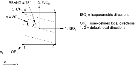
As an example, a user-defined local coordinate system is used to define skewed rebar in
a shell element (skew angle ), and the output value of
RBANG is 75°, as illustrated in Figure 18:
Figure 18. RBANG measurement for skew
rebar defined relative to user-defined local coordinate directions.
The rebars are located at the midsurface of the shell. Output variable
RBANG is measured from the second
isoparametric direction to the rebar. If the first isoparametric direction were chosen
instead, output variable RBANG would
report an angle of 165°.
Visualizing Rebar Orientation and Results in Rebar
Abaqus/CAE does not support visualization of element-based rebar or rebar results. Abaqus/CAE does support visualization of rebar defined as described in Defining Reinforcement.