Orientations

You must assign a name to each orientation definition. This name is used by various features to refer to the orientation definition.

ORIENTATION, NAME=name

Any module: ToolsDatum: Type: CSYS: select any method, and click OK: Name: name

In a model defined in terms of an assembly of part instances, you can define a local orientation at the part, part instance, or assembly level. An orientation defined at the part or part instance level is rotated according to the positioning data given for each instance of that part (or for the part instance). This includes the case when an orientation is defined using a distribution. See Assembly Definition and Distribution Definition.

A two-stage process is used to define the local system directly.

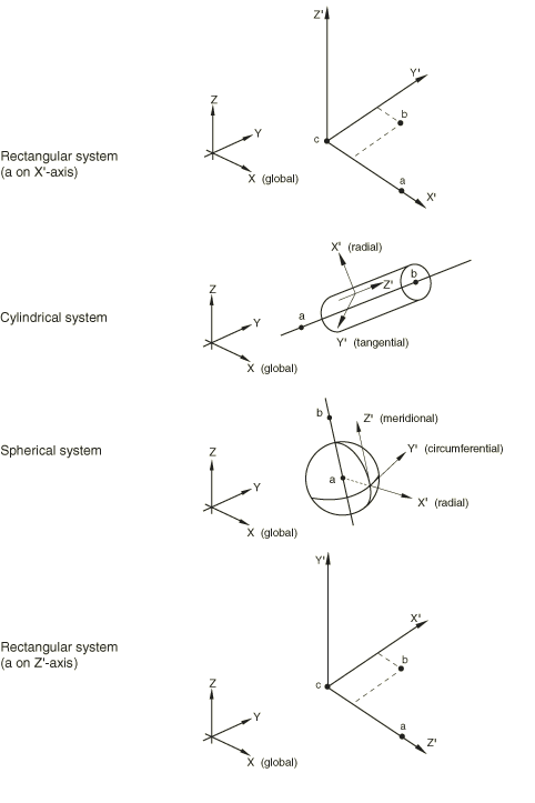
1. You define the local coordinate system at the particular location at which it is required. You can select a rectangular, cylindrical, or spherical coordinate system. The coordinate system is defined in terms of points a, b, and c, as shown in Figure 1. You can select the method for defining points a, b, and c, as described below.

   Figure 1. Orientation systems.
   
   

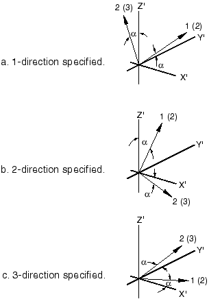
2. Optionally, you can specify an additional rotation by identifying one of these local directions ($X^{\prime }$, $Y^{\prime }$, or $Z^{\prime }$) as a rotation axis and giving a rotation, in degrees, about that axis. The local system is then rotated through this angle about the specified axis. This method of defining a local system is required for contact surfaces in Abaqus/Standard, shells, membranes, gasket elements, and when the orientation is associated with a composite solid section. The additional rotation is illustrated in Figure 2.

   Figure 2. Specifying rotation about a local axis for shell elements, membrane elements, gasket elements (in parentheses), composite solids (in parentheses), and contact surfaces in Abaqus/Standard.
   
   

   The local coordinate system for composite solids is indicated by $X^{\prime }$, $Y^{\prime }$, and $Z^{\prime }$. The local coordinate system for other element types is indicated by 1, 2, and 3; the axis labels in parentheses are oriented for gasket elements.

You can model multiscale materials with fiber dispersion (see Specifying a Second-Order Orientation Tensor in Abaqus/Explicit and Specifying a Second-Order Orientation Tensor in Abaqus/Standard) or short-fiber reinforced linear composites (see Defining the Elasticity of a Short-Fiber Reinforced Composite).

In Abaqus/Explicit, you must specify the second-order tensor that characterizes the fiber dispersion as part of a local orientation system definition if the values vary spatially. In addition, when modeling short-fiber reinforced linear composites, you must specify a local orientation system that is aligned with the principal directions of the second-order tensor.

When specifying a spatially varying second-order tensor in Abaqus/Standard, you can either specify the distribution of the second-order tensor as part of a local orientation system definition or as part of a material definition (see Specifying a Second-Order Orientation Tensor in Abaqus/Standard).

ORIENTATION, DISPERSION

When modeling anisotropic hyperelastic materials with an invariant-based formulation (see Invariant-Based Formulation) you must define the local directions that characterize each family of fibers. These directions need not be orthogonal in the initial configuration. You can specify these local directions with respect to an orthogonal orientation system at a material point. Up to three local directions can be specified as part of the definition of a local orientation system. The local directions can be output as field variables to the output database (see Output).

ORIENTATION, LOCAL DIRECTIONS=N

In general, the yarn directions in a fabric material might not be orthogonal to each other in the reference configuration (see Fabric Material Behavior). You can specify these local directions with respect to the in-plane axes of an orthogonal orientation system at a material point. Both the local directions and the orthogonal system are defined together as a single orientation definition. If the local directions are not specified, these directions are assumed to match the in-plane axes of the orthogonal system defined. The local direction might not remain orthogonal with deformation. Abaqus updates the local directions with deformation and computes the nominal strains along these directions and the angle between them (the fabric shear strain). The constitutive behavior for the fabric defines the nominal stresses in the local system in terms of the fabric strain. The local directions can be output as field variables to the output database (see Output).

ORIENTATION, LOCAL DIRECTIONS=2

In some cases the simplest way to specify a local system is by means of a user subroutine. User subroutine ORIENT is provided in Abaqus/Standard. In this case the user subroutine is called each time that an orientation definition is needed. In a model defined in terms of an assembly of part instances, the local directions defined by user subroutine ORIENT must be defined relative to the coordinate system of the assembly.

ORIENTATION, NAME=name, SYSTEM=USER

Because the orientation is independent of the material definition and they can both be referenced in any element property definition, the ability to describe complex structural components (such as laminated composite shells) is quite general and straightforward to use.

An orientation definition can be used as often as needed and with different material or element type definitions; for example, it can be used for different layers of a shell where the orientation is the same.

In large-displacement analysis a user-defined orientation rotates with the average rigid body motion of the material point, the rigid body when the orientation is used with ROTARYI elements, the first node of the joint in JOINTC elements, the pipeline edge for pipe-soil interaction elements, the appropriate surface for contact in Abaqus/Standard, or the reference node when the orientation is used with coupling constraints. However, when an orientation is defined for spring, dashpot, or gasket elements in Abaqus/Standard, the local directions always remain fixed in space.

Because the material directions rotate with the average rigid body motion at a material point, using anisotropic elasticity to model a material that is not truly a continuum can give significant errors if shear deformation is large. For example, an individual fiber in a reinforcing belt of a tire can shear relatively easily with respect to fibers in other directions. The fibers rotate with the actual deformation of the material point and not with the average rigid body motion. In this case the anisotropic behavior is better modeled with rebars or as a fabric material. The fabric material model in Abaqus/Explicit tracks the current yarn directions as local directions with respect to the orthogonal coordinate system.

When a user-defined orientation is used with two-dimensional solid elements such as plane stress, plane strain, or torsionless axisymmetric elements, the orientation must redefine only the X- and Y-directions: the third direction must remain unchanged (Z-direction for plane strain and plane stress elements, $\theta$ -direction for axisymmetric elements). When a user-defined orientation is used for material behavior with axisymmetric elements with twist, all three directions can be redefined. For axisymmetric elements, including the CGAX and CAXA families of elements, the global 1-, 2-, and 3-directions are the radial, axial, and hoop directions, respectively. Cylindrical or spherical orientations might be appropriate for axisymmetric elements only if the local $Z^{\prime }$ -direction is in the global 3-, or hoop, direction.

When a user-defined orientation is used with shell, continuum solid shell, membrane, or gasket elements or with contact surfaces, Abaqus first rotates and then projects the orientation system onto the element or contact surface using the algorithm described in this section.

Abaqus first rotates (through the additional rotation angle) the user-defined local coordinate system about the specified rotation axis. If you do not specify a rotation axis or an additional angle, Abaqus will by default use the local 1-axis and a rotation of 0°. After the rotation, Abaqus follows a cyclic permutation (1, 2, 3) of the axes and projects the axis following the axis for additional rotation onto the contact surface or onto the surface of the element to form the local material 1-direction (or the local material 2-direction for gaskets). The remaining material direction is then defined by the cross product of the element normal and the projected direction. Thus, for example:

1. If you choose the user-defined 1-axis as the axis for additional rotation, Abaqus projects the 2-axis onto the element or contact surface. This will be local direction 1 for contact surfaces, shells, and membranes and local direction 2 for gaskets.

2. Abaqus takes the positive element or contact surface normal as the local 3-direction for contact surfaces, shells, and membranes and the local 1-direction for gaskets.

3. Abaqus computes the local 2-direction (3-direction for gaskets) by taking the cross product of the element or contact surface normal and the local 1-direction (2-direction for gaskets), such that the three local axes form an orthonormal, right-handed local coordinate system.

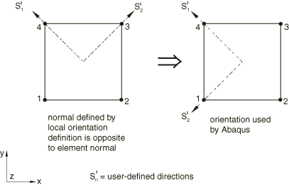
When the axis for additional rotation points in a direction that is opposite to the element or contact surface normal, the local 2-direction (3-direction for gaskets) is reversed with respect to the corresponding user-defined axis; see Figure 3. This does not apply in the case of an orientation used to define rebars; see below.

Figure 3. The local 3-direction (1-direction for gaskets) will be in the same direction as the element or contact surface normal.

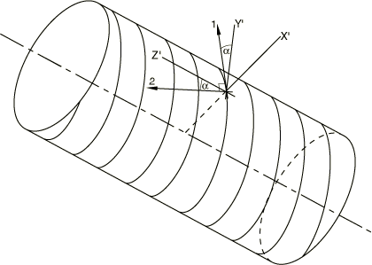
As an example, the orientation of the spiral-wound layer of the cylindrical shell shown in Figure 4 would be given by defining a cylindrical coordinate system and then specifying the rotation axis as the 1-axis and giving the rotation angle $\alpha$ (in degrees). The local 1- and 2-directions for material property specification and material calculations are then those indicated in the figure.

Figure 4. Spiral-wound cylindrical shell layer: material orientation example.

The projected directions are most easily understood when the axis for additional rotation is approximately perpendicular to the element or contact surface.

To define a spatially varying local coordinate system directly, you can specify the additional angle of rotation on an element-by-element basis using a distribution. See Distribution Definition.

There are two ways in which a user-defined orientation can be used in the section definition of a laminated shell. In each case the name referenced in the shell section definition is the name of the user-defined orientation.

The first is to associate the user-defined orientation with the entire composite shell section definition. Then each layer's orientation angle can be given relative to this section orientation (or the default shell coordinate directions if no section orientation is used). The angle is given as an additional rotation about the shell normal after the orientation directions are projected onto the shell surface. Section forces (available only from Abaqus/Standard) are given in the local system specified for the section.

The second is to specify the name of each layer's orientation separately; this method allows different orientation definitions to be referenced for the different layers. Section forces and strains are still reported in the local orientation defined for the entire section (or the default shell coordinate directions if no section orientation is used). The individual layer orientations are used for material calculations and for output of stress and strain.

See Using a Shell Section Integrated during the Analysis to Define the Section Behavior and Using a General Shell Section to Define the Section Behavior for more information.

When a user-defined orientation is used with composite solid elements (available only in Abaqus/Standard), one of the local directions must be identified as the axis for additional rotation. There are two ways in which this orientation can be used with a composite solid section definition to specify the material orientation for individual layers. In each case the name referenced in the solid section definition is the name of the user-defined orientation.

The first is to associate the user-defined orientation with the entire composite solid section definition. Then each layer's orientation angle can be given relative to this section orientation. The angle is given as an additional rotation about the local direction defined as the axis for additional rotation. For continuum solid shell elements, the angle is given as an additional rotation about the element normal after the orientation directions are projected onto the element midsurface.

The second is to specify the name of each layer's orientation separately; this method allows different orientation definitions to be referenced for the different layers. (In this case any user-defined orientation associated with the entire solid section will be ignored.) For continuum solid shell elements, each layer's orientation is projected onto the element midsurface.

See Defining the Elements Section Properties for more information.

An arbitrary user-defined orientation can be defined for pipe-soil interaction elements (available only in Abaqus/Standard). In a large-displacement analysis the local orientation system rotates with the rigid body motion of the underlying pipeline. In a small-displacement analysis the local system is defined by the initial geometry of the PSI element and remains fixed in space during the analysis.

See Beam Element Cross-Section Orientation for information on defining local material directions for beams, frames, or trusses.

The fill and the warp yarn directions in the fabric plane are allowed to rotate with respect to each other under shear deformations (see Fabric Material Behavior). The current yarn directions are tracked with respect to the orthogonal coordinate system that also rotates with the material.

When a user-defined orientation is used to define a joint system orientation for the jointed material model available in Abaqus/Standard (see Jointed Material Model), only the local coordinate system need be defined. It is assumed that the first direction is the direction normal to the plane of the joint and the other directions are in the plane of the joint. An additional axis of rotation cannot be used.

A user-defined orientation must be used to define the local directions for certain connection types used to define connector elements (see Connection Types).

A user-defined orientation can be used with SPRING1, SPRING2, DASHPOT1, DASHPOT2, JOINTC, JOINT2D, JOINT3D, and ROTARYI elements to provide a local system for defining the direction of action of such elements. Points a, b, and c (see Figure 1) cannot be defined by giving local node numbers when the orientation is used for these elements. If you do not specify an axis for additional rotation, the local 1-direction with no additional rotation will be chosen as the default.

User-defined orientations can be used in Abaqus/Standard to define the local coordinate systems in which constraint directions are specified for a kinematic coupling constraint (see Kinematic Coupling Constraints). In this case you cannot define points a, b, and c by giving local node numbers (see Figure 1).

User-defined orientations can be used to define the local coordinate systems in which surface-based coupling constraint directions are specified (see Coupling Constraints). In this case you cannot define points a, b, and c by giving local node numbers (see Figure 1).

A user-defined orientation can be used in Abaqus/Standard to define a local system of directions along which the inertia relief loads are computed (see Inertia Relief). In this case you cannot define points a, b, and c by giving local node numbers (see Figure 1).

User-defined orientations can be used in Abaqus to define the local coordinate systems in which the loading directions for distributed general tractions, shear tractions, and general edge loads are specified. See Distributed Loads.

Spatially varying local coordinate systems (for material definitions, material calculations, and output) defined with a distribution can be applied only to solid continuum, membrane (in Abaqus/Standard), and shell elements. See Solid (Continuum) Elements, Membrane Elements, Using a Shell Section Integrated during the Analysis to Define the Section Behavior, and Using a General Shell Section to Define the Section Behavior.