Mean-Field Homogenization

Specifying Constituent Properties for a Composite Material

In multiscale material modeling, each composite material consists of one matrix material and one or more inclusions including voids. In Abaqus/Explicit, the composite material must consist of one matrix material and only one inclusion; the inclusion material must be linear elastic with constant properties, and the matrix material can be only linear elastic or elastic-plastic with isotropic hardening.

Input File Usage

Use the following option to define the properties of the matrix in the composite:

CONSTITUENT, TYPE=MATRIX

Use the following option to define the properties of a nonvoid inclusion in the composite:

CONSTITUENT, TYPE=INCLUSION

Use the following option to define the properties of a void inclusion in the composite:

CONSTITUENT, TYPE=VOID

Mean-Field Homogenization for Linear Elastic Composites

The mean-field strain and stress in each phase I is defined as

{\bar{σ}}_{I} = {〈 σ 〉}_{I}

{\bar{ϵ}}_{I} = {〈 ϵ 〉}_{I},

where

〈 f 〉 = \frac{1}{V} \int_{V}^{} f d V .

The averaged macro fields can be written as

〈 • 〉 = v_{f}^{M} {〈 • 〉}_{M} + \sum_{I = 1}^{N} v_{f}^{I} {〈 • 〉}_{I},

where $v_{f}^{M}$ is the volume fraction of the matrix phase and $v_{f}^{I}$ is the volume fraction of the inclusion phase. For the single-inclusion case, if all the constituents are linear elastic, the strain in the inclusion is related to the strain in the matrix through a concentration tensor $A$ .

{〈 ϵ 〉}_{I} = A {〈 ϵ 〉}_{M} .

The strain and stress in the inclusion/matrix can also be related to the macro strain/stress through the strain/stress concentration tensor $B_{I, M}^{ϵ}$ and $B_{I, M}^{σ}$ :

{〈 ϵ 〉}_{I, M} = B_{I, M}^{ϵ} 〈 ϵ 〉 .

{〈 σ 〉}_{I, M} = B_{I, M}^{σ} 〈 σ 〉 .

The form of the concentration tensor defines the homogenization methods below.

Voigt and Reuss Models

The simplest mean-field homogenization formulations are the Voigt and Reuss models. These models do not take into account the shape or the orientation of the inclusions; however, they provide upper and lower bounds of the macro stiffness modulus and, therefore, can be used for validation. The Voigt model is also used in a two-step approach to model composites with multiple inclusions.

The Voigt model assumes uniform strain in the composite ${〈 ϵ 〉}_{I} = {〈 ϵ 〉}_{M}$ , which gives

A = I .

The Reuss model assumes uniform stress in the composite ${〈 σ 〉}_{I} = {〈 σ 〉}_{M}$ , which gives

A = C_{I}^{- 1} C_{M},

where $C_{M}$ is the stiffness of the matrix and $C_{I}$ is the stiffness of the inclusion.

Input File Usage

Use the following option to specify the Voigt model as the homogenization method:

 MEAN FIELD HOMOGENIZATION, FORMULATION=VOIGT

Use the following option to specify the Reuss model as the homogenization method:

 MEAN FIELD HOMOGENIZATION, FORMULATION=REUSS

Micromechanical Models for Unidirectional Composites

The Chamis model (Chamis, 1989) and Composite Cylinder Assemblage (CCA) model (Christensen, 1979) are micromechanical homogenization models developed and validated for unidirectional composites.

With the composite stiffness known from the micromechanical models, the concentration tensor can be computed using

A = \frac{v_{f}^{M}}{v_{f}^{I}} {(C_{C} - C_{I})}^{- 1} (C - C_{M}),

where

C_{C}

is the composite stiffness,

C_{M}

is the stiffness of the matrix, and

C_{I}

is the stiffness of the inclusion.

Input File Usage

Use the following option to specify the Chamis model as the homogenization method:

 MEAN FIELD HOMOGENIZATION, FORMULATION=CHAMIS

Use the following option to specify the CCA model as the homogenization method:

 MEAN FIELD HOMOGENIZATION, FORMULATION=CCA

Eshelby-Based Models

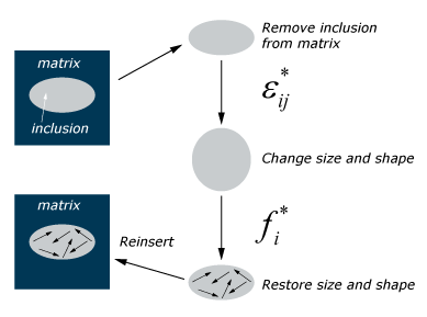
The more sophisticated mean-field homogenizations are based on Eshelby's solution. In his 1957 paper (Eshelby, 1957), Eshelby solved a single-inclusion problem described in Figure 1.

Eshelby found that the strain inside the constrained ellipsoid is uniform and given by

ϵ (x) = E : ϵ^{*},

where $x$ represents a point inside the inclusion and $ϵ^{*}$ is the eigenstrain. The Eshelby tensor (E) is a function of the stiffness of the matrix and also the shape and orientation of the inclusion. To calculate Eshelby's tensor usually involves numerical integration over the surface of the ellipsoidal inclusion; however, analytical solutions are available (Mura, 1987) for simple shapes such as a sphere, cylinder, penny, oblate, and prolate. Based on Eshelby's solution, the following models are proposed based on different assumptions about the properties of the outer material surrounding the inclusions.

Mori-Tanaka Model

The Mori-Tanaka formulation assumes that each inclusion behaves like an isolated inclusion and the strain in the matrix is considered as the far-field strain. Therefore, the concentration tensor can be written as

A = {[E : (C_{M}^{- 1} C_{I} - I) + I]}^{- 1} .

Input File Usage

 MEAN FIELD HOMOGENIZATION, FORMULATION=MT

Inverse Mori-Tanaka Model

The inverse Mori-Tanaka formulation assumes a high volume fraction of the inclusion and permutes the properties of the matrix and inclusion in a single inclusion problem, which gives

A = {[E : (C_{I}^{- 1} C_{M} - I) + I]}^{- 1} .

Input File Usage

 MEAN FIELD HOMOGENIZATION, FORMULATION=INVERSED MT

Balanced Model

The Mori-Tanaka and inverse Mori-Tanaka formulations give the upper and lower bounds of the composite stiffness for low and high volume fractions. The balanced formulation is the interpolative formulation, which can be written as

H_{1} = {[E : (C_{M}^{- 1} C_{I} - I) + I]}^{- 1},

H_{2} = {[E : (C_{I}^{- 1} C_{M} - I) + I]}^{- 1},

A = {[(1 - φ) H_{1}^{- 1} + φ H_{2}^{- 1}]}^{- 1},

where $φ$ is the smooth interpolation function proposed by Lielens (1999)

φ = \frac{1}{2} v_{f}^{I} (1 + v_{f}^{I}) .

Input File Usage

MEAN FIELD HOMOGENIZATION, FORMULATION=BALANCED

User-Defined Concentration Tensor

You can define the concentration tensor $A$ directly by specifying all of its components. The user-defined concentration tensor must be defined in the local coordinate system of the inclusion. You can use homogenization models other than those listed above, calibration from experimental results, or FE-RVE models to obtain the value of the concentration tensor.

Input File Usage

Use the following option to define the fourth-order strain concentration tensor used to calculate the strain in a constituent:

CONCENTRATION TENSOR, TYPE=STRAIN (default)

Use the following option to define the second-order conductivity concentration tensor used to calculate the temperature gradient in a constituent:

CONCENTRATION TENSOR, TYPE=CONDUCTIVITY

Mean-Field Homogenization for Thermal Properties

Mean-field homogenization can also be used to compute effective thermal properties and micro-level thermal fields of the constituents.

Conductivity

The effective conductivity of composite materials can also be computed using Eshelby's single-inclusion method described in Mean-Field Homogenization for Linear Elastic Composites. For example, Mori-Tanaka method gives the following conductivity concentration tensor

A^{C} = {[E^{C} : (k_{M}^{- 1} k_{I} - I) + I]}^{- 1} .

where

E^{C}

is the modified 3x3 second-order Eshelby's tensor and

k_{I, M}

are second-order conductivity tensor of the constituents.

The relationship between the temperature gradient in the constituents is given by

{〈 \nabla θ 〉}_{I} = A^{C} {〈 \nabla θ 〉}_{M} .

and the macro-level temperature gradient is the volume-averaged temperature gradient of the constituents. Chamis and CCA formulations are not supported for conductivity.

Specific Heat and Latent Heat

The specific heat and latent heat of the composite can be compute using the mass-averaged value of the constituents.

Incremental Mean-Field Homogenization for Nonlinear Composites

An incremental linearization approach is used to extend the homogenization models to composites with nonlinear behavior. The tangent stiffness matrix is used in place of the linear elastic modulus to compute the concentration tensor $A$

Δ ϵ_{I} = A Δ ϵ_{M} .

Since the tangent matrix is not constant in the nonlinear case and is usually a function of the strain, iterations are performed to guarantee a converged solution of the strain increment in each constituent.

Isotropization Methods

Analytical expression of Eshelby's tensor is available only if the inclusions are ellipsoidal and the matrix material is isotropic or transversely isotropic. For matrix materials that are anisotropic, using the stiffness directly to compute the Eshelby's tensor can result in stiffer prediction for the composite behavior (Doghri, 2003). The isotropic part of the tangent stiffness matrix can generally be written as

C^{i s o} = 3 K I^{v o l} + 2 G I^{d e v},

where $K$ is the bulk modulus and $G$ is the shear modulus. $I^{v o l}$ and $I^{d e v}$ are the volumetric and deviatoric part of the fourth-order identity tensor. The method used to extract the isotropic part of the stiffness matrix is not unique, and the accuracy of the prediction varies depending on the properties of the matrix material.

General Method

The general method is the most common isotropization method, and it extracts the isotropic part using

K = \frac{1}{3} I^{v o l} : : C^{a n i},

G = \frac{1}{10} I^{d e v} : : C^{a n i} .

The general method can be used for any anisotropic tangent matrix. This method is the default isotropization method.

Input File Usage

CONSTITUENT

Spectral Method

The spectral isotropization method can be used if isotropic hardening is defined in the matrix material (Doghri, 2003). The isotropic part of the tangent matrix is given by

K = K_{e},

G = G_{e} (1 - \frac{3 G_{e}}{3 G_{e} + \frac{d σ^{0}}{d {\bar{ϵ}}^{p l}} ({\bar{ϵ}}^{p l})}),

where $K_{e}$ is the elastic bulk modulus, $G_{e}$ is the elastic shear modulus, $σ^{0} ({\bar{ϵ}}^{p l})$ is the yield stress, and ${\bar{ϵ}}^{p l}$ is the equivalent plastic strain.

Input File Usage

CONSTITUENT, ISOTROPIZATION COEFFICIENT=1.0

Modified Spectral Method

For matrix materials with significant softening after yielding, both the general method and the spectral method might give predictions that are too stiff. The modified spectral method proposed by Selmi et. al. (Selmi, 2011) improves the accuracy of the spectral method by evaluating the derivative of the yield stress at a larger equivalent plastic strain

K = K_{e},

G = k_{G} G_{e} (1 - \frac{3 G_{e}}{3 G_{e} + \frac{d σ^{0}}{d {\bar{ϵ}}^{p l}} (k_{p} {\bar{ϵ}}^{p l} + k_{s})}),

where $k_{G}$ , $k_{p}$ , and $k_{s}$ are the isotropization parameters. You can calibrate these parameters by comparing the mean-field solution to experimental data or to FE-RVE solutions. The isotropization parameters are irrelevant if the constituent does not have plastic behavior.

Input File Usage

Use the following option when all the parameters are constant and $k_{p}$ is the only parameter with a nondefault value:

CONSTITUENT, ISOTROPIZATION COEFFICIENT=isotropization coefficient

Use the following options to define temperature- or field-dependent isotropization parameters:

CONSTITUENT
ISOTROPIZATION PARAMETERS

Isotropic Projection

Options are available to use the isotropic projection of the tangent matrix to compute different parts of the concentration tensor. For better predictions, Doghri et al. (Doghri, 2010) recommended the following:

If the general method is used, only Eshelby's tensor is computed with the isotropic projection.
If the spectral/modified spectral method is used, Hill's tensor given by $P = E : C_{M}^{- 1}$ is computed with the isotropic projection.

It is possible that some choices can lead to unphysical prediction of microlevel strain resulting in unstable material behavior in the composite. In addition, in Abaqus/Standard analyses, the tangent stiffness matrix for the composite might lose its symmetry after homogenization; therefore, you must use the unsymmetric solver to achieve convergence.

Input File Usage

Use the following option to use the isotropic projection of the matrix stiffness to compute all parts of the concentration tensor by default:

 MEAN FIELD HOMOGENIZATION, ISOTROPIZATION=ALLISO

Use the following option to use the isotropic projection of the matrix stiffness to compute only Eshelby's tensor:

 MEAN FIELD HOMOGENIZATION, ISOTROPIZATION=E-ISO

Use the following option to use the isotropic projection of the matrix stiffness to compute Hill's tensor:

 MEAN FIELD HOMOGENIZATION, ISOTROPIZATION=P-ISO

Multistep Homogenization

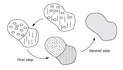
For composites with multiple inclusions, a multistep homogenization approach is used, as shown in Figure 2. The composite is decomposed into "grains," with each grain containing one inclusion family and the matrix. The inclusions in each family have the same material properties, aspect ratio, and orientation. In the first step homogenization is performed in each grain using the user-specified formulation; in the second step, the Voigt formulation is used to compute the properties of the overall composite.

An alternative approach is to use the Mori-Tanaka scheme in both the first and the second step, assuming the average strain in the matrix is uniform across all grains. This approach is equivalent to the direct Mori-Tanaka approach proposed by Benveniste (Benveniste et al., 1991). In an Abaqus/Standard analysis, the second approach has the drawback that it might result in an unsymmetric effective modulus when the inclusions are misaligned and nonisotropic. In such cases, use of the unsymmetric solver might be necessary.

Abaqus/Explicit analyses only support one matrix and one inclusion material. For composites with dispersed fiber directions (see Specifying a Second-Order Orientation Tensor in Abaqus/Explicit), the direct Mori-Tanaka approach is used.

Input File Usage

Use the following option to use the Voigt formulation in the second step homogenization for the multiphase composite:

MEAN FIELD HOMOGENIZATION, UNIFORM MATRIX STRAIN=NO

Use the following option to use the direct Mori-Tanaka formulation for the multiphase composite, assuming the average strain in the matrix is uniform across all grains:

MEAN FIELD HOMOGENIZATION, UNIFORM MATRIX STRAIN=YES

Specifying the Microstructure of the Composite

You can specify the microstructure of the composite by giving the shape, volume fraction, aspect ratio, and fiber orientation of each constituent. You can use a distribution to define the volume fraction, aspect ratio, and the orientation tensor (see Distribution Definition).

The orientation tensor can be used only with three-dimensional solid elements.

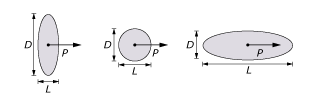
Specifying the Shape, Volume Fraction, and Aspect Ratio

The volume fraction and aspect ratio can be specified as spatial distributions. The aspect ratio is given by $L / D$ as shown in Figure 3.

The aspect ratio of a spherical inclusion is 1.0, and the aspect ratio of a cylindrical inclusion is infinity; therefore, you do not need to specify the aspect ratio in these cases.

Input File Usage

Use the following option to specify a prolate-shaped inclusion ( $L > D$ ):

CONSTITUENT, SHAPE=PROLATE
volume fraction, aspect ratio,

Use the following option to specify an oblate-shaped inclusion ( $L < D$ ):

CONSTITUENT, SHAPE=OBLATE
volume fraction, aspect ratio,

Use the following option to specify a penny-shaped inclusion ( $L ≪ D$ ):

CONSTITUENT, SHAPE=PENNY
volume fraction, aspect ratio,

Use the following option to specify a spherical inclusion:

CONSTITUENT, SHAPE=SPHERE
volume fraction,

Use the following option to specify a continuous cylindrical inclusion with a circular cross-section:

CONSTITUENT, SHAPE=CYLINDER
volume fraction,

Use the following option to specify a continuous cylindrical inclusion with an elliptical cross-section:

CONSTITUENT, SHAPE=ELLIPTIC CYLINDER
volume fraction,  $a_{2} / a_{3}$

Here $a_{2}$ and $a_{3}$ are the radii of the elliptical cross-section along the axis in the local 2- and 3-directions.

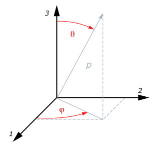
Specifying a Fixed Orientation for the Inclusion and Void Phases

By default, the orientation of the inclusion or void phase is fixed and is aligned with the x-axis of the local coordinate system specified in the section definition. You can specify a different orientation by giving the three components of the orientation vector in the local coordinate system, as shown in Figure 4. The components of the orientation unit vector, $p$ , are

\begin{matrix} p_{1} & = & \sin θ \cos φ, \\ p_{2} & = & \sin θ \sin φ, \\ p_{3} & = & \cos θ . \end{matrix}

The local 3-direction of the inclusion (void included) is the projection of the local z-axis defined in the section onto the surface normal to the inclusion orientation (1-direction). If the local z-axis is within 0.1 degree of being parallel to the 1-direction, the local 3-direction is the projection of the local y-axis onto the surface. The local 2-direction is then at right angles to the local 3-direction, so that the local 2-direction, local 3-direction, and the inclusion orientation (1-direction) form a right-handed set. The local 2 and 3 directions are relevant only if the shape of the inclusion (void included) is an elliptical cylinder.

Input File Usage

Use the following option to specify a fixed fiber orientation:

CONSTITUENT, DIRECTION=FIXED
 ,  ,  $p_{1}, p_{2}, p_{3}$

Specifying a Second-Order Orientation Tensor in Abaqus/Standard

For composites containing short fibers, a second-order orientation tensor, $a$ , is usually used to describe the dispersion of the fiber orientation

a_{i j} = \oint p_{i} p_{j} Ψ (p) d p,

where $\oint d p = \int_{φ = 0}^{2 π} \int_{θ = 0}^{π} \sin θ d θ d φ$ is the integral over the surface of the unit sphere (all possible directions of $p$ ) and $Ψ (p)$ is the orientation distribution function (ODF). The spatial distribution of the orientation tensor is usually given by injection molding software and can be used directly to compute the effective moduli of the composite material that is linear elastic. If the material is nonlinear, the average fields given by $〈 f 〉 = \oint f (p) Ψ (p) d p$ must be computed during the analysis, and the ODF is required to calculate the integral. When only the second-order orientation is available, Abaqus recovers the ODF using the approach proposed by Onat and Leckie (1988)

Ψ (p) ≃ \frac{1}{4 π} + \frac{15}{8 π} b_{i j} f_{i j} (p) + \frac{315}{32 π} B_{i j k l} F_{i j k l} (p),

for three-dimensional orientations, where $f_{i j}$ and $F_{i j k l}$ are the tensor basis functions

f_{i j} (p) = p_{i} p_{j} - \frac{1}{3} δ_{i j},

F_{i j k l}^{} = p_{i} p_{j} p_{k} p_{l} - \frac{1}{7} (p_{i} {p_{j} δ}_{k l} + {p_{i} p_{k}}_{} δ_{j l} + p_{i} p_{l} δ_{j k} + p_{k} p_{l} δ_{i j} + p_{j} p_{l} δ_{i k} + p_{j} p_{k} δ_{i l}) + \frac{1}{35} (δ_{i j} δ_{k l} + δ_{i k} δ_{j l} + δ_{i l} δ_{j k}),

and $b_{i j}$ and $B_{i j k l}$ are the deviatoric versions of the orientation tensors

b_{i j} = a_{i j} - \frac{1}{3} δ_{i j},

B_{i j k l}^{} = A_{i j k l} - \frac{1}{7} (a_{i j} δ_{k l} + a_{i k} δ_{j l} + a_{i l} δ_{j k} + a_{k l} δ_{i j} + a_{j l} δ_{i k} + a_{j k} δ_{i l}) + \frac{1}{35} (δ_{i j} δ_{k l} + δ_{i k} δ_{j l} + δ_{i l} δ_{j k}) .

The fourth-order orientation tensor is required during the ODF reconstruction. It is computed using a closure approximation, which is a formula that approximates the fourth-order tensor in terms of the known second-order tensor. A popular closure approximation is the hybrid closure approximation proposed by Advani and Tucker (1987), which is constructed using the interpolation of linear and quadratic closure approximation

A_{i j k l}^{h} = (1 - α) A_{i j k l}^{l} + α A_{i j k l}^{q},

where the linear closure is given by

A_{i j k l}^{l} = - \frac{1}{35} (δ_{i j} δ_{k l} + δ_{i k} δ_{j l} + δ_{i l} δ_{j k}) + \frac{1}{7} (a_{i j} δ_{k l} + a_{i k} δ_{j l} + a_{i l} δ_{j k} + a_{k l} δ_{i j} + a_{j l} δ_{i k} + a_{j k} δ_{i l}),

and the quadratic closure is given by

A_{i j k l}^{q} = a_{i j}^{} a_{k l} .

The weight function is defined as $α = 1 - 27 \det (a)$ for three-dimensional orientations.

Other available closure approximations are the orthotropic smooth approximation (Advani and Tucker, 1987), the orthotropic fitted (ORF) approximation (Cintra and Tucker, 1995), and the orthotropic equaivalent of the natural (ORE) approximation (VerWeyst, 1998).

Only one constituent in the composite is allowed to have orientations specified with the second-order orientation tensor.

Taking into account the symmetry of the ODF $Ψ (p) = Ψ (- p)$ , we compute the integral $\oint f (p) Ψ (p) d p$ numerically as follows:

\oint f (p) Ψ (p) d p ≃ {2 \sum}_{I = 1}^{N} \sum_{I = 1}^{N} f (θ_{I}, φ_{J}) Ψ (θ_{I}, φ_{J}) \sin (θ_{I}) Δ θ Δ φ,

where $Δ θ = Δ φ = \frac{π}{N}$ and $θ_{I} = I Δ θ, φ_{J} = J Δ φ$ . The numerical integral is computed by subdividing the macro point into $N \times N$ subdomains, with each subdomain having the same fiber orientation $p = p (θ_{I}, φ_{J})$ . Then a multistep homogenization (as described in Figure 2) is used to compute the macrolevel solutions. The ODF is more accurately recovered if a large value of N is used; however, the computational cost and memory usage also increases substantially.

When the fiber direction is random in the three-dimensional space, the second-order orientation tensor is $a_{i j} = \frac{1}{3} δ_{i j}$ , and the ODF is constant across all subdomains.

When the direct Mori-Tanaka homogenization approach is used, the fiber response can be calculated either individually in each subdomain or just once using the averaged state over all subdomains. In both cases only the averaged fiber state is available for output. The maximum principal direction of the second-order orientation tensor is used as the 1-direction of the local coordinate system for the inclusion.

In composites where the fiber material is linear elastic with uniform moduli across all pseudo-grains, if we assume uniform matrix strain inside the composite, homogenization and strain partitioning can be simplified. Instead of computing the integrals numerically, Abaqus/Standard uses the following equation to compute the orientation averaging terms, $C^{a v g} = \oint C (p) Ψ (p) d p$ :

C_{i j k l}^{a v g} = C_{1} a_{i j k l} + C_{2} (a_{i j} δ_{k l} + a_{k l} δ_{i j}) + C_{3} (a_{i k} δ_{j l} + a_{i l} δ_{j k} + a_{j l} δ_{i k} + a_{j k} δ_{i l}) + C_{4} δ_{i j} δ_{k l} + C_{5} (δ_{i k} δ_{j l} + δ_{i l} δ_{j k}),

where

C_{1}

,

C_{2}

,

C_{3}

,

C_{4}

, and

C_{5}

are the five constants of the tensor that is transversely isotropic. ODF reconstruction is not necessary and is not performed.

Input File Usage

Use the following option to specify the fiber orientation using a second-order tensor:

CONSTITUENT, DIRECTION=ORIENTATION TENSOR
 , ,  $a_{11}, a_{22}, a_{33}, a_{12}, a_{13}, a_{23}$

Use the following option to specify a random fiber orientation:

CONSTITUENT, DIRECTION=RANDOM3D

Use the following option to specify the number of subdivisions used to compute the surface integral:

MEAN FIELD HOMOGENIZATION, ANGLE SUBDIVISIONS=N

Use the following option to compute the fiber response individually in each subdomain:

CONSTITUENT, RESPONSE=GRANULAR (default)

Use the following options to compute the average response of the fiber directly when using the direct Mori-Tanaka homogenization approach:

MEAN FIELD HOMOGENIZATION, UNIFORM MATRIX STRAIN=YES
CONSTITUENT, RESPONSE=AVERAGE

Use the following option to compute the ODFs using the orthotropic fitted (ORF) closure approximation:

MEAN FIELD HOMOGENIZATION, CLOSURE=FITTED

Use the following option to compute the ODFs using the orthotropic equivalent of the natural (ORE) closure approximation:

MEAN FIELD HOMOGENIZATION, CLOSURE=ORE

Use the following option to compute the ODFs using the hybrid closure approximation:

MEAN FIELD HOMOGENIZATION, CLOSURE=HYBRID

Use the following option to compute the ODFs using the quadratic closure approximation:

MEAN FIELD HOMOGENIZATION, CLOSURE=QUADRATIC

Use the following option to compute the ODFs using the orthotropic smooth closure approximation:

MEAN FIELD HOMOGENIZATION, CLOSURE=SMOOTH

Use the following option to compute the orientation averaging directly:

MEAN FIELD HOMOGENIZATION, ORIENTATION AVERAGING=DIRECT, UNIFORM MATRIX STRAIN=YES

Specifying a Second-Order Orientation Tensor in Abaqus/Explicit

In Abaqus/Explicit, when a second-order orientation tensor, $a$ , is used to specify the dispersion of the fiber material, the direct Mori-Tanaka approach is used. Because the fiber material can be only linear elastic with uniform moduli across all pseudo-grains, ODF reconstruction is not performed and orientation averaging terms are computed directly.

The second-order orientation tensor is specified in the orientation definition of the section where the multiscale material is assigned.

Input File Usage

Use the following option to specify the fiber orientation using a second-order tensor:

CONSTITUENT, DIRECTION=ORIENTATION TENSOR

Use the following option to specify the components of a second-order tensor in the orientation definition:

ORIENTATION, DISPERSION

Composites with Thermal Expansion

Composites with thermal expansion are supported only in Abaqus/Standard.

The effective thermal expansion coefficient tensor can be computed using Levin's theorem (2):

〈 α 〉 = \sum_{I = 1}^{N} v_{f}^{I} α_{I} B_{I}^{σ} + v_{f}^{M} α_{M} B_{M}^{σ},

where

α_{I, M}

are the thermal expansion coefficients of the constituents,

N

is the total number of inclusions, and

B_{I, M}^{σ}

are the stress concentration tensors defined in Mean-Field Homogenization for Linear Elastic Composites.

In the presence of thermal strains due to a temperature change, the averaged strain/stress in each constituent can be written as:

{〈 ϵ 〉}_{I, M} = B_{I, M}^{ϵ} 〈 ϵ 〉 + B_{I, M}^{T} Δ T .

The relationship between $B_{I, M}^{ϵ}$ and $B_{I, M}^{T}$ can be established through superposition of the two problems to achieve the condition $〈 ϵ 〉 = 0$ with $Δ T \neq 0$ (3).

Problem I solves a uniform stress field ${〈 σ 〉}_{I} = {〈 σ 〉}_{M} = 〈 σ 〉$ under the condition $Δ T \neq 0$ while assuming ${ϵ^{'} = 〈 ϵ^{'} 〉}_{I} = {〈 ϵ^{'} 〉}_{M}$ . The solution to problem I gives

ϵ^{'} = {(C_{I} - C_{M})}^{- 1} (β_{I} - β_{M}) Δ T,

where

β_{I, M} = C_{I, M} α_{I, M}

.

Problem II is purely mechanical assuming $Δ T = 0$ . Solving $〈 ϵ 〉 = 0$ gives the solution

{〈 ϵ^{''} 〉}_{I, M} = - B_{I, M}^{ϵ} ϵ^{'} .

By superimposing the constituent strain solutions from problem I and problem II, we get

{〈 ϵ 〉}_{I, M} = {〈 ϵ^{'} 〉}_{I, M} + {〈 ϵ^{''} 〉}_{I, M} = (I - B_{I, M}^{ϵ}) {(C_{I} - C_{M})}^{- 1} (β_{I} - β_{M}) Δ T,

which results in the relationship between

B_{I, M}^{T}

and

B_{I, M}^{ϵ}

below

B_{I, M}^{T} = (I - B_{I, M}^{ϵ}) {(C_{I} - C_{M})}^{- 1} (β_{I} - β_{M}) .

Thermal expansion is supported only for plane strain and three-dimensional solid elements.

Composites with Viscoelasticity

Composites with viscoelasticity are supported only in Abaqus/Standard.

When one or more constituents have viscoelasticity defined in the time domain, the homogenization approach described above is no longer appropriate because it does not take into account the relaxation of stress with time. However, similar homogenization can be performed in the frequency domain, and homogenized properties of the composite in the time domain can be computed using homogenized properties at different frequencies. This homogenization approach is applicable only when the viscoelasticity in the constituents is defined in the time domain using a Prony series expansion and includes the following steps:

The shear and bulk moduli of all the constituents are transformed to the frequency domain using Fourier transforms (see details in Prony Series Parameters).
The mean-field homogenization is performed in the frequency domain the same way as discussed above, with the exception that the moduli are complex numbers instead of real numbers. The real part of the composite modulus is the storage modulus, $C^{s}$ , and the imaginary part is the loss modulus, $C^{l}$ .
Assuming the time response of the composite can be written in a similar form as that in the constituents where viscoelasticity is defined using a Prony series expansion
$g_{i j} (t) = 1 - \sum_{k = 1, N} g_{k} (1 - e^{- t / τ_{k}}),$
where $g_{i j} (t) = C_{i j} (t) / C_{i j}^{0}$ and $C_{i j}^{0}$ is the instantaneous elastic modulus of the composite, the homogenized storage modulus of the composite, $C^{s}$ , can be written in the frequency domain as follows:
$C_{i j}^{s} (ω) = C_{i j}^{0} [1 - \sum_{k = 1, N} \frac{g_{k}}{1 + τ_{k}^{2} ω^{2}}] .$
The parameters $τ_{k}$ are selected to be equally spaced numbers on a logarithmic scale in the range $[τ_{\min}, τ_{\max}]$ . $τ_{\min}$ and $τ_{\max}$ are the minimum and maximum frequencies used to define the viscoelasticity in all constituents. The parameters $g_{k}$ are computed through a least-squares curve fit at frequencies $ω_{l} = 1 / τ_{l}$ $(l = 1, N)$ .

You can only specify the thermorheologically simple temperature effect in the matrix material. The composite is assumed to inherit the same temperature effect as the matrix material.

Other limitations include:

The inverse Mori-Tanaka and balanced homogenization formulations are not supported when you use the orientation tensor to define the direction of the inclusion.
When you use the orientation tensor to define the direction of the inclusion, the elasticity specified in the inclusion material must satisfy the transversely isotropic condition, and no other inclusions can be defined in the composite.
You cannot use the orientation tensor to define the direction of the inclusion in which viscoelasticity is defined.
Distributions other than distributions of the orientation tensor are not allowed in the material definition.
Temperature and field variable dependencies are allowed to define the elasticity of the matrix material only, and only one inclusion is allowed in this case.
Other than viscoelasticity, only the following properties are supported in the inclusion material:
1. Conductivity
2. Density
3. Elasticity
4. Thermal expansion
5. Specific heat
Other than viscoelasticity, only the following properties are supported in the matrix material:
1. Conductivity
2. Density
3. Elasticity
4. Thermal expansion
5. Specific heat
6. Cure properties

Because the multiscale material is replaced by a composite with prehomogenized properties, the microlevel output is not available. Other than viscoelasticity, Abaqus/Standard also computes the homogenized values of all the other supported properties.

Composites Curing

Mean-field homogenization can be used to model composite behavior during a curing process (Curing Processes in Polymers). Similar to composites with viscoelasticity, a multiscale material is replaced by a composite with prehomogenized properties. The same limitations described in Composites with Viscoelasticity also apply.

The composite inherits the following properties from the matrix material definition:

Cure kinetics
Cure max conversion
Cure glass transition temperature

Mean-field homogenization is used to compute the following cure properties for the composite:

Cure heat generation. The specific heat of the reaction is computed using mass-averaged value of the constituents.
Cure shrinkage. Levin's theorem is used to compute the effective thermal expansion coefficient (Composites with Thermal Expansion) and to compute the effective cure shrinkage coefficient of the composite.

Composites with Damage

When damage and failure are defined at the constituent level, the damage in each constituent contributes to the overall damage in an indirect way through stress averaging and strain partitioning. As the stiffness of the constituent decreases, the strain increment in this constituent is likely to increase based on the formulation of the homogenization. In reality, the damage behavior of each constituent is likely to interact with each other and affect the overall damage behavior of the composite; therefore, you might need to specify an additional damage variable, $D$ , for the composite. At any time during the analysis, the stress tensor of the composite is given by

σ = (1 - D) \bar{σ},

where $\bar{σ} = \sum_{i} v_{i}^{f} σ_{i}$ , and $σ_{i} = (1 - D_{i}) {\bar{σ}}_{i}$ is the effective stress of the constituent.

You can choose to combine the damage variables, $D_{i}$ , in all constituents to get the overall damage behavior of the composite. The overall damage variable, $D$ , can be computed as the maximum of $D_{i}$ :

D = \max {D_{i}},

or you can choose to combine the damage variables in a multiplicative sense:

D = 1 - \prod_{i} (1 - D_{i}) .

You can also specify $D$ using user subroutine UDAMAGEMF. In addition, you can specify a separate damage variable, $d_{i}^{int}$ , for each constituent. This variable is used to account for the additional contribution to the overall damage behavior due to interaction (for example, a fiber material might buckle more easily if cracks start to develop in the matrix material) as follows:

σ = (1 - D) \sum_{i} v_{i}^{f} (1 - d_{i}^{int}) σ_{i} .

Input File Usage

Use the following option to specify that $D_{i}$ contributes to $D$ in a maximum sense:

MEAN FIELD DAMAGE, DEGRADATION=MAXIMUM

Use the following option to specify that $D_{i}$ contributes to $D$ in a multiplicative sense:

MEAN FIELD DAMAGE, DEGRADATION=MULTIPLICATIVE

Use the following option to specify a user-defined damage behavior for the composite:

MEAN FIELD DAMAGE, DEGRADATION=USER

Example

This simple example illustrates how to define a multiscale material.

The name of the multiscale material is COMPOSITE. The material consists of one inclusion material MAT2 embedded in the matrix material MAT1. The shape of the inclusion is prolate. The Mori-Tanaka homogenization method is used. The inclusion has a volume fraction of $v_{f}^{}$ and an aspect ratio of $a r$ . The direction of the inclusion is fixed and defined with a vector $(p_{1}, p_{2}, p_{3})$ . The name of the matrix is MATRIX_MAT1, and the name of the inclusion is FIBER_MAT2.

Input file template

MATERIAL, NAME=MAT1
…
MATERIAL, NAME=MAT2
…
MATERIAL, NAME=COMPOSITE
MEAN FIELD HOMOGENIZATION, FORMULATION=MT
CONSTITUENT, TYPE=MATRIX, MATERIAL=MAT1, NAME=MATRIX_MAT1
CONSTITUENT, TYPE=INCLUSION, MATERIAL=MAT2, NAME=FIBER_MAT2, SHAPE=PROLATE, DIRECTION=FIXED
 $v_{f}^{}$ ,  $a r$ ,  $p_{1}$ ,  $p_{2}$ ,  $p_{3}$

Elements

In Abaqus/Standard the multiscale material model can be used with

three-dimensional solid elements, including stress/displacement elements, diffusive heat transfer elements, and coupled temperature-displacement elements;
two-dimensional solid elements (stress/displacement only);
membrane elements;
three-dimensional conventional shell elements (stress/displacement only); and
continuum shell elements (stress/displacement only).

In Abaqus/Standard additional plane stress iterations are included for two-dimensional plane stress elements and shell elements.

In Abaqus/Explicit the multiscale material model can be used only with three-dimensional solid stress/displacement elements.

Hybrid elements and incompatible mode elements are not supported.

Output

By default, the output variables are macrolevel results. In addition, you can also request microlevel output. The name of the constituent is appended to the end of the output variable.

For composites reinforced with dispersed short fibers, the fiber output variables are computed in the local system with the local fiber direction as the maximum principal direction of the orientation tensor. The matrix output is available only if the direct Mori-Tanaka homogenization approach is used. Otherwise, only averaged stress and strain are available. If plasticity is specified in the matrix material, averaged plastic strains are also available. The same matrix output limitation also applies to composites reinforced with multiple fiber families.

Microlevel strain output is not available in Abaqus/Explicit.

Input File Usage

Use the following options to request field output for the constituents:

OUTPUT, FIELD
ELEMENT OUTPUT, MICROMECHANICS

Use the following options to request history output for the constituents:

OUTPUT, HISTORY
ELEMENT OUTPUT, MICROMECHANICS

References

Advani, S., and C. Tucker, “The Use of Tensors to Describe and Predict Fiber Orientation in Short Fiber Composites,” Journal of Rheology, vol. 31 (8), pp. 751–784, 1987.
Levin, V.M., “On the Coefficients of Thermal Expansion of Heterogeneous Materials,” Mechanics of Solids, vol. 2, pp. 58–61, 1967.
Benveniste, Y., and G. J. Dvorak, “On a Correspondance Between Mechanical and Thermal Effects in Two-Phase Composites,” Micromechanics and Inohomogeneity, pp. 65–81, 1990.
Benveniste, Y., G. J. Dvorak, and T. Chen, “On Diagonal and Elastic Symmetry of the Approximate Effective Stiffness Tensor of Heterogeneous Media,” Journal of the Mechanics and Physics of Solids, vol. 39(7), pp. 927–946, 1991.
Chamis, C.C., “Mechanics of Composite Materials: Past, Present and Future,” Journal of Composites Technology and Research, vol. 11, pp. 3–14, 1989.
Christensen, R.M., “Solutions for Effective Shear Properties in Three Phase Sphere and Cylinder Models,” Journal of the Mechanics and Physics of Solids, vol. 27, pp. 315–330, 1979.
Cintra, J., and C. Tucker, “Orthotropic Closure Approximations for Flow-Induced Fiber Orientation,” Journal of Rheology, vol. 39, pp. 1095–1122, 1995.
Doghri, I., I. Adam, and N. Bilger, “Mean-Field Homogenization of Elasto-Viscoplastic Composites Based on a General Incrementally Affine Linearization Method,” International Journal of Plasticity, pp. 219–238, 2010.
Doghri, I., and A. Ouaar, “Homogenization of Two-Phase Elasto-Plastic Composite Materials and Structures. Study of Tangent Operators, Cyclic Plasticity and Numerical Algorithms,” International Journal of Solids and Structures, vol. 40(7), pp. 1681–1712, 2003.
Eshelby, J. D., “The Determination of the Elastic Field of an Ellipsoidal Inclusion and Related Problems,” Proceedings of the Royal Society of London, pp. 376–396, 1957.
Kammoun, S., L. Brassart, G. Robert, I. Doghri, and L. Delannay, “Micromechanical Modeling of Short Glass-Fiber Reinforced Thermoplastics-Isotropic Damage of Pseudograins,” American Institute of Physics Conference Proceedings 1353, pp. 974–977, 2011.
Lielens, G., “Micro-Macro Modeling of Structured Materials,” PhD Thesis Universite Catholique de Louvain Belgium, 1999.
Mura, T., Micromechanics of Defects in Solids, MARTINUS NIJHOFF Publishers , 1987.
Onat, E.T., and F.A. Leckie, “Representation of Mechanical Behavior in the Presence of Changing Internal Structure,” Journal of Applied Mechanics, vol. 55(1), pp. 1–10, 1988.
Pierard, O., and I. Doghri, “An Enhanced Affine Formulation and the Corresponding Numerical Algorithms for the Mean-Field Homogenization of Elasto-Viscoplastic Composites,” International Journal of Plasticity, pp. 131–157, 2006.
Selmi, A., I. Doghri, and L. Adam, “Micromechanical Simulations of Biaxial Yield, Hardening and Plastic Flow in Short Glass Fiber Reinforced Polyamide,” International Journal of Mechanical Sciences, vol. 53(9), pp. 696–706, 2011.
VerWeyst, B.E., “Numerical Predictions of Flow-Induced Fiber Orientation in 3-D Geometries,” Ph.D. thesis, University of Illinois at Urbana-Champaign, 1998.