Coupling Constraints

Surface-Based Coupling Definitions

The surface-based coupling constraint in Abaqus provides coupling between a reference node and a group of surface nodes. Surface-based coupling constraints are useful for transmitting loads or imposing conditions on a surface region of a part. The loads or imposed conditions can be specified directly, or they can arise from discrete connections, such as spotwelds, between surfaces. Use of a surface-based coupling rather than applying a load or imposing a condition at a single surface node reduces sensitivity of simulation results to mesh details.

Key differences between the available surface-based coupling types include whether rigidity is imposed among nodes involved in the coupling and which degrees of freedom are associated with the coupling.

Kinematic coupling acts on mechanical degrees of freedom and imposes rigidity on the system of nodes involved.
Distributing coupling acts on mechanical degrees of freedom and does not impose rigidity; instead, the reference node displacement and rotation correspond to a weighted-average motion among surface nodes involved in the coupling (taking into consideration any offset of the reference node from the center of the surface nodes).

The constraint equations associated with distributing coupling have the effect of distributing a force or moment acting on the reference node among the surface nodes of the coupling. Uniform coupling imposes uniformity of nonmechanical degrees of freedom among the coupled nodes. A uniform coupling constraint can act on the same reference node and surface as a kinematic or distributing constraint because different (nonmechanical versus mechanical) degrees of freedom are involved.

Surface-based coupling provides functionality similar to the kinematic coupling constraint element and the distributing coupling element types (DCOUP2D, DCOUP3D) in Abaqus/Standard; however, it has a surface-based user interface. Abaqus selects the group of surface nodes automatically by specifying a surface and an optional influence region. The procedure used to define the coupling nodes is discussed below.

Abaqus automatically calculates the weight factors associated with averaging of a distributing coupling constraint if the surface is an element-based surface. In such a case, the weight factors are based on the tributary area at each coupling node, except for a surface along a shell edge, where the weight factors are based on the tributary edge length. In addition, you can modify the distributing weight factors using one of several weighting methods, which allow the forces transferred to the coupling nodes to vary inversely with the radial distance from the reference node.

Typical Applications

You can employ surface-based coupling constraints effectively in the following situations:

To distribute loads on a model, where the load distribution can be described with a moment-of-inertia expression. Examples of such cases include the classic bolt-pattern and weld-pattern distribution expressions.
To apply dimensionality transitions between continuum and structural elements. For example, a distributing coupling allows flexible coupling between structural and solid elements.
To model end conditions. For example, modeling a rigid end plate or modeling plane sections of a solid to remain planar can be done easily with a kinematic coupling definition.
To simplify modeling of complex constraints. In a kinematic coupling definition the degrees of freedom that participate in the constraint can be selected individually in a local coordinate system.
To model interactions with other constraints, such as connector elements. For example, a hinged part can be modeled more realistically by two distributing coupling definitions, whose reference nodes are connected by a hinge connector element. The load transfer then occurs between two “clouds” of nodes, rather than between two single nodes. Substructure analysis of a one-piston engine model illustrates this use of connector elements with coupling constraints to model a one-piston engine.
To constrain nonmechanical degrees of freedom of the nodes on a surface to a uniform value with a uniform coupling. The kinematic and distributing couplings act on mechanical degrees of freedom (displacements and rotations) only. A uniform coupling constraint can be used together with a kinematic or distributing coupling constraints (such as the ones shown in Figure 1 or Figure 2), or independently.

Defining a Surface-Based Coupling Constraint

Defining a coupling constraint requires the specification of the reference node (also called the constraint control point), the coupling surface, and the constraint type. The coupling constraint associates the reference node with the nodes of the coupling surface. A name must be assigned to the constraint and can be used in postprocessing with Abaqus/CAE. A node number or node set name can be specified for the reference node. When the reference node set contains multiple nodes, you should specify a radius of influence to avoid overconstraint issues. The reference node for a kinematic coupling constraint has both translational and rotational degrees of freedom. The surface on which the coupling nodes are located can be node-based; element-based; or, in Abaqus/Explicit, a combination of both surface types. You can specify an optional radius of influence to limit the coupling nodes to a specific region on the surface. Details on how coupling nodes are defined by specifying an influence region are discussed below.

The constraint type can be either kinematic or distributing, as discussed below.

Input File Usage

Use the following options:

COUPLING, CONSTRAINT NAME=name, REF NODE=n, 
SURFACE=surface
KINEMATIC,  DISTRIBUTING, or UNIFORM

Abaqus/CAE Usage

Interaction module: Create Constraint: Coupling: Coupling type:
Kinematic, Continuum distributing, or Structural distributing

Specifying a Region of Influence

By default, coupling nodes belonging to the entire surface are selected for the coupling definition. You can limit the coupling nodes to lie within a spherical region centered about the reference node by defining a radius of influence.

The procedure by which coupling nodes are selected for the constraint definition depends on the surface type:

For a node-based surface, all the nodes defined by the surface definition that fall within the influence region are selected for the coupling definitions.
For an element-based surface, the surface facets that are either fully or partially inscribed by the influence region are determined. All nodes belonging to these facets, whether or not these nodes fall within the influence region, are selected for the coupling nodes. When the influence radius is less than the distance to the closest coupling node, Abaqus selects all nodes belonging to the closest facet. If the projection of the reference node on the surface falls on an edge or a vertex of multiple facets, all nodes belonging to these facets adjoining the edge or vertex are included in the coupling definition. In the case where the influence radius is less than the distance to the closest coupling node, adjacent surface faces must have consistent normal directions; otherwise, Abaqus issues an error message.
A distributing coupling constraint must include at least two coupling nodes. If fewer than two coupling nodes are found, Abaqus issues an error message during input file preprocessing.

Input File Usage

COUPLING, CONSTRAINT NAME=name, REF NODE=n, 
SURFACE=surface, INFLUENCE RADIUS=r

Abaqus/CAE Usage

Interaction module: Create Constraint: Coupling: Influence radius: Specify

Kinematic Coupling Constraints

Kinematic coupling constrains the motion of the coupling nodes to the rigid body motion of the reference node. The constraint can be applied to user-specified degrees of freedom at the coupling nodes with respect to the global or a local coordinate system. Only required degrees of freedoms are activated at the reference node. If no displacement degree of freedom is constrained, the displacement degrees of freedom at the reference node may not be activated.

Kinematic constraints are imposed by eliminating degrees of freedom at the coupling nodes. In Abaqus/Standard once any combination of displacement degrees of freedom at a coupling node is constrained, additional displacement constraints—such as MPCs, boundary conditions, or other kinematic coupling definitions—cannot be applied to any coupling node involved in a kinematic coupling constraint. The same limitation applies for rotational degrees of freedom. This restriction does not apply in Abaqus/Explicit. See About Kinematic Constraints for more information.

Input File Usage

Use both of the following options to define a kinematic coupling constraint:

COUPLING
KINEMATIC
first dof, last dof

For example, the following coupling constraint is used to constrain degrees of freedom 1, 2, and 6 on surface surfA to reference node 1000:

COUPLING, CONSTRAINT NAME=C1, REF NODE=1000, SURFACE=surfA
KINEMATIC
1, 2
6,

Abaqus/CAE Usage

Interaction module: Create Constraint: Coupling: Coupling type: Kinematic: toggle on the degrees of freedom

Translational Degrees of Freedom

Translational degrees of freedom are constrained by eliminating the specified degrees of freedom at the coupling nodes. When all translational degrees of freedom are specified, the coupling nodes follow the rigid body motion of the reference node.

Rotational Degrees of Freedom

Rotational degrees of freedom are constrained by eliminating the specified degrees of freedom at the coupling nodes.

All combinations of selected rotational degrees of freedom result in rotational behavior identical to existing MPC types:

Selection of three rotational degrees of freedom along with three displacement degrees of freedom is equivalent to MPC type BEAM.
Selection of two rotational degrees of freedom is equivalent to MPC type REVOLUTE in Abaqus/Standard.
Selection of one rotational degree of freedom is equivalent to MPC type UNIVERSAL in Abaqus/Standard.

In Abaqus/Standard, internal nodes are created by the kinematic coupling to enforce the constraints that are equivalent to MPC types REVOLUTE and UNIVERSAL. These nodes have the same degrees of freedom as the additional nodes used in these MPC types and are included in the residual check for nonlinear analysis.

Specifying a Local Coordinate System

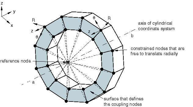
The kinematic coupling constraint can be specified with respect to a local coordinate system instead of the global coordinate system (see Orientations). Figure 1 illustrates the use of a local coordinate system to constrain all but the radial translation degrees of freedom of the coupling nodes to the reference node. In this example, a local cylindrical coordinate system is defined that has its axis coincident with the structure's axis. The coupling node constraints are then specified in this local coordinate system.

Input File Usage

COUPLING, ORIENTATION=local

For example, the following input is used to specify the kinematic coupling constraint shown in Figure 1:

ORIENTATION, SYSTEM=CYLINDRICAL, NAME=COUPLEAXIS
0.0, -1.0, 0.0, 0.0, 1.0, 0.0
COUPLING, REF NODE=500, SURFACE=Endcap, 
ORIENTATION=COUPLEAXIS
KINEMATIC
2, 3

Abaqus/CAE Usage

Interaction module: Create Constraint: Coupling: Edit: select local coordinate system

Constraint Direction and Finite Rotation

In geometrically nonlinear analysis steps the coordinate system in which the constrained degrees of freedom are specified will rotate with the reference node regardless of whether the constrained degrees of freedom are specified in the global coordinate system or in a local coordinate system.

Thermal Expansion of a Kinematic Coupling

In Abaqus/Standard a kinematic coupling can experience expansion due to a temperature increase. Each coupled node expands along the line that joins the node to the reference node. The magnitude of the expansion depends on the distance of the coupled node from the reference node. The temperature change for computing the expansion is the average of the temperature change at the node and the temperature change at the reference node. The temperature change at any node is the difference between the initial temperature of the node and the current temperature of the node. You must provide the value of the thermal expansion coefficient so that Abaqus/Standard can compute the expansion. Thermal expansion can be used only when temperature is a field variable.

Input File Usage

KINEMATIC, ALPHA=thermal_expansion_coeff

Abaqus/CAE Usage

Interaction module: Create Constraint: Coupling: Coupling type:
Kinematic: Thermal expansion coefficient

Distributing Coupling Constraints

Distributing coupling constrains translation and rotation of the reference node to the average motion of the coupling cloud nodes. The cloud nodes will follow the motion of the reference node in an average sense, but, unlike kinematic coupling, deformation can occur among cloud nodes.

The rotational coupling constraint enforces that the rotation of the reference node equals an average rotation measure of the cloud nodes. In Abaqus/Standard this averaging considers translations and rotations (if rotational degrees of freedom are present) of the cloud nodes by default. Typically, this averaging heavily weights the average "swirling" of the cloud due to coupling node translations, with coupling node rotations having a small influence. Coupling node rotations have a greater effect on the rotational constraint if the cloud nodes are approximately colinear. The rotational coupling constraint for Abaqus/Explicit only considers the average swirling of coupling node translations.

The translational coupling constraint is such that translation of the weighted center of the cloud corresponds to the average translation of the cloud nodes. By default, the reference node translation follows the weighted center translation plus the effect of rotation of a rigid arm from the weighted center to the reference node. This rigid-arm rotation corresponds to the reference node rotation. Optionally, cloud node rotational degrees of freedom can participate in an additional offset term for the translational coupling constraint such that the reference node remains close to a shell surface during bending.

Forces and moments acting on the reference node are typically distributed as a nodal force distribution among cloud nodes, plus (often small) moments acting at any cloud nodes whose rotations influence translational or rotational constraints. The coupling constraints distribute loads such that the resultants of forces and moments at the cloud nodes are equivalent to the forces and moments at the reference node. For cases of more than a few cloud nodes, the distribution of forces/moments is not determined by equilibrium alone, and distributing weight factors are used to define the force distribution.

Input File Usage

DISTRIBUTING

Abaqus/CAE Usage

Interaction module: Create Constraint: Coupling: Continuum distributing

Neglecting Cloud Rotations in Rotational Coupling Constraints

In Abaqus/Standard you can optionally neglect cloud node rotational degrees of freedom in rotational coupling constraints. In Abaqus/Explicit they are always neglected. In this case, the rotation of the reference node matches the average “swirling” of the cloud associated with cloud node translations.

If cloud rotations do not participate in the rotational coupling constraint, moments at the reference node are transmitted as a pure force distribution among the cloud nodes. Therefore, when the cloud node arrangement is colinear, the constraint is not capable of transmitting all components of a moment at the reference node. Specifically, the moment component that is parallel to the colinear coupling node arrangement is not transmitted. When this case arises, Abaqus issues a warning message that identifies the axis about which the element will not transmit a moment.

Input File Usage

DISTRIBUTING, ROTATIONAL COUPLING=CONTINUUM

Abaqus/CAE Usage

A nondefault option for Abaqus/Standard to neglect cloud rotations in a rotational constraint for distributing coupling is not supported in Abaqus/CAE.

Optional Offset Associated with Bending

Cloud node rotations can optionally be considered in translational coupling constraints such that the reference node remains near a shell surface as it bends. For this coupling method to be active, all rotation degrees of freedom at all coupling nodes must be active (as is the case when the constraint is applied to a shell surface) and the constraints must be specified in all degrees of freedom (the default). In addition, for the constraint to be meaningful, the local (or global) z-axis used in the constraint should be such that it is parallel to the average normal direction of the constrained surface.

The translational constraint enforces a rigid beam connection between the reference node and a moving point that remains in the vicinity of the constrained surface at all times. The location of this moving point is determined by the approximate current curvature of the surface, the current location of the weighted center of the coupling nodes, and the z-axis used in the constraint.

Use of this option is independent of whether or not cloud node rotations influence rotational coupling constraints.

Input File Usage

DISTRIBUTING, COUPLING=STRUCTURAL

Abaqus/CAE Usage

Interaction module: Create Constraint: Coupling: Structural distributing

Releasing Components of the Rotational Coupling Constraint

You can optionally specify which degrees of freedom of the coupling constraint to constrain. Only rotational components can be released. All available translational degrees of freedom at the reference node are always coupled to the average translation of the coupling nodes and must be included in the degrees of freedom to constrain. One rotational constraint component can be released in a two-dimensional analysis. One, two, or three rotational constraint components can be released in a three-dimensional analysis. You can specify the rotational constraint directions in the global coordinate system or in a local coordinate system.

In a three-dimensional Abaqus/Standard analysis, if all three rotational constraints are released by constraining only degrees of freedom 1 through 3, only translation degrees of freedom are activated on the reference node. If only one or two rotation degrees of freedom are released, all three rotation degrees of freedom are activated at the reference node. In this case you must ensure that proper constraints have been placed on the unconstrained rotation degrees of freedom to avoid numerical singularities. Most often this is accomplished by using boundary conditions or by attaching the reference node to an element such as a beam or shell that provides rotational stiffness to the unconstrained rotational degrees of freedom.

In Abaqus/Explicit releasing one or more of the rotational constraints can lead to significant computational performance degradation. This is also the case when other constraints intersect the cloud of coupling nodes. In these cases, the degradation in performance is particularly noticeable when a large number of such distributed couplings are present in the model or when the size of the constrained “cloud” is large. Therefore, when the modeling conditions mentioned above are encountered, the size of the coupling nodes cloud is limited to 1000.

The following modeling technique can be used to alleviate rotational constraint issues: constrain all rotations in the distributed coupling and use an appropriate connector element at the reference node (such as REVOLUTE, HINGE, CARDAN, or BUSHING) to model released moments at the coupling's reference node. This technique also has the advantage of being able to specify finite compliance such as elasticity, plasticity, or damage in the “released” rotational component.

In geometrically nonlinear analysis steps the coordinate system of the degrees of freedom that define the rotational constraint release rotates with the reference node regardless of whether the global coordinate system or a local coordinate system is used.

Input File Usage

DISTRIBUTING
first dof, last dof

If no degrees of freedom are specified, all available degrees of freedom are coupled. If you specify one or more rotation degrees of freedom but not all available translation degrees of freedom, Abaqus issues a warning message and adds all available translation degrees of freedom to the constraint.

For example, the following coupling constraint is used to constrain degrees of freedom 1–5 on the reference node 1000 to the average translation and rotation of surface surfA:

COUPLING, CONSTRAINT NAME=C1, REF NODE=1000, SURFACE=surfA
DISTRIBUTING
1, 5

In this example the moment constraint between the reference node and the coupling nodes will be released in the 6-direction but will be enforced in the 4- and 5-directions. This provides a “revolute-like” rotation connection between the reference node and the coupling nodes (see General Multi-Point Constraints).

Abaqus/CAE Usage

Interaction module: Create Constraint: Coupling: Coupling type: Continuum distributing or Structural distributing: toggle on the rotational degrees of freedom

Abaqus/CAE automatically constrains the translational degrees of freedom.

Node-Based Surface

User-defined weight factors are used for node-based surfaces. The cross-sectional areas specified in the surface definition are used as the weight factors (see Node-Based Surface Definition).

Element-Based Surface

For element-based surfaces the weight factors are calculated by Abaqus. The default weight distribution is based on the tributary surface area at each coupling node, except for a surface along a shell edge where the weight distribution is based on the tributary edge length. The procedure used to calculate the default weight factors is designed to ensure that if a radius of influence is prescribed, the default weight distribution varies smoothly with the influence radius.

Calculating the Default Distributing Weight Factors

The procedure to calculate the distributing weight factors depends on whether or not an influence radius is specified.

If no influence radius is specified, the entire surface is used in the coupling definition. In this case all nodes located on the surface are included in the coupling definition and the distributing weight factor at each coupling node is equal to the tributary surface area.
If an influence radius is specified, the default distributing weight factors at the coupling nodes are calculated as follows:
1. A “participation factor” is calculated for each surface facet. The participation factor is defined below.
2. The tributary nodal area (or tributary edge length along a shell edge) at each facet node is computed and is multiplied by the facet participation factor.
3. The coupling node distributing weight factor is computed as the sum of the corresponding facet nodal areas (calculated above) for all joining facets.

Calculating the Facet Participation Factor

The participation factor defines the proportion of the facet's area that contributes to the distributing weight factors when an influence radius is specified. The participation factor varies between zero and one.

To define the participation factor, the distance of the facet node closest to the reference node, $r_{m i n}$ , and the distance of the facet node farthest from the reference node, $r_{m a x}$ , are calculated.

If $r_{m a x} \leq r_{i n f l}$ , where $r_{i n f l}$ is the influence radius, all facet nodes lie within the influence region; and a participation factor of one is used.
If $r_{m i n} \geq r_{i n f l}$ , none of the facet nodes lie within the influence region; and the participation factor is set to zero.
If $r_{m a x} > r_{i n f l}$ , the facet is partially inscribed in the influence region; and the facet is assigned a participation factor equal to $(r_{i n f l} - r_{m i n}) / (r_{m a x} - r_{m i n})$ .

If all coupling nodes fall outside the influence radius (that is, $r_{m i n} > r_{i n f l}$ for all facets), Abaqus selects all nodes belonging to the closest facets (as outlined under “Specifying a region of influence”) and uses a participation factor equal to one.

Weighting Methods

You can modify the default weight distribution defined above. Various weighting methods are provided that monotonically decrease with radial distance from the reference node. For each case the default weight distribution that is based on the tributary surface area (or tributary edge length along a shell edge) is scaled by the weight factor $w_{i}$ . If the weighting method is not specified, a uniform weighting method is used in which all weight factors are equal to 1.0.

Linearly Decreasing Weight Distribution

A linearly decreasing weighting scheme

w_{i} = 1 - \frac{r_{i}}{r_{0}},

where $w_{i}$ is the weight factor at coupling node i, $r_{i}$ is the coupling node radial distance from the reference node, and $r_{0}$ is the distance to the furthest coupling node.

Input File Usage

DISTRIBUTING, WEIGHTING METHOD=LINEAR

Abaqus/CAE Usage

Interaction module: Create Constraint: Coupling: Coupling type: Continuum distributing or Structural distributing: Weighting method: Linear

Quadratic Polynomial Weight Distribution

A quadratic polynomial weight distribution defined by

w_{i} = 1 - {(\frac{r_{i}}{r_{0}})}^{2} .

Input File Usage

DISTRIBUTING, WEIGHTING METHOD=QUADRATIC

Abaqus/CAE Usage

Interaction module: Create Constraint: Coupling: Coupling type: Continuum distributing or Structural distributing: Weighting method: Quadratic

Monotonically Decreasing Weight Distribution

A monotonically decreasing weight distribution according to the cubic polynomial

w_{i} = 1 - 3 {(\frac{r_{i}}{r_{0}})}^{2} + 2 {(\frac{r_{i}}{r_{0}})}^{3} .

Input File Usage

DISTRIBUTING, WEIGHTING METHOD=CUBIC

Abaqus/CAE Usage

Interaction module: Create Constraint: Coupling: Coupling type: Continuum distributing or Structural distributing: Weighting method: Cubic

Processing of Unattached Nodes

Cloud nodes that have no stiffness cause numerical singularities in Abaqus/Standard analyses. You can guide Abaqus/Standard to provide proper management of such nodes. By default, Abaqus/Standard allows nodes that are not attached to any user elements. You can direct Abaqus/Standard to remove nodes that are not attached to any user elements or to issue an error message. You should keep unattached nodes if they derive their stiffness by being main nodes to other nodes that have stiffness.

Input File Usage

Use the following option to direct Abaqus/Standard to allow nodes that are not attached to any user elements (default):

DISTRIBUTING, FREE NODES=ALLOW

Use the following option to direct Abaqus/Standard to remove nodes that are not attached to any user elements:

DISTRIBUTING, FREE NODES=REMOVE

Use the following option to direct Abaqus/Standard to issue an error message:

DISTRIBUTING, FREE NODES=ERROR

Abaqus/CAE Usage

Directing Abaqus/Standard to remove or allow nodes that are not attached to any user elements is not supported in Abaqus/CAE.

Specifying a Local Coordinate System

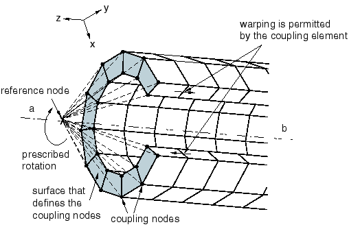
The distributing coupling constraint can be specified with respect to a local coordinate system instead of the global coordinate system (see Orientations). Figure 2 illustrates the use of a local coordinate system to release the moment constraints between the reference node and the coupling nodes in the local 4- and 6-directions, providing a “universal-like” rotation connection. In this example, a local rectangular coordinate system is defined that has its local y-axis coincident with the global z-axis. The moment constraint is specified in this local coordinate system.

Input File Usage

COUPLING, ORIENTATION=local

For example, the following input is used to specify the distributing coupling constraint shown in Figure 2:

ORIENTATION, SYSTEM=RECTANGULAR, NAME=COUPLEAXIS
0.0, 1.0, 0.0, 0.0, 0.0, 1.0
COUPLING, REF NODE=500, SURFACE=Endcap, 
ORIENTATION=COUPLEAXIS
DISTRIBUTING
1, 3
5, 5

Abaqus/CAE Usage

Interaction module: Create Constraint: Coupling: Edit: select local coordinate system

Uniform Coupling Constraints

Uniform coupling constraints impose uniformity in temperature or other nonmechanical degrees of freedom among the coupled nodes. You can prescribe the value of the uniform field with a boundary condition at the reference node, or the evolving value of the uniform field can be determined by the simulation.

For a uniform coupling constraint, the reference node acts as the independent (or main) node and the surface nodes act as dependent (or secondary) nodes. A dependent degree of freedom of the uniform coupling constraint cannot also be constrained with a boundary condition or act as a secondary degree of freedom of another MPC in Abaqus/Standard.

If a reference node of a uniform coupling constraint is not involved in other couplings or elements, that node will have only the degree of freedom type associated with the uniform coupling constraint (such as temperature), even if surface nodes of the uniform coupling constraint have displacement degrees of freedom. For example, a force load cannot be applied to such a reference node.

It is common for the reference node of a uniform coupling constraint to act as a reference node of a kinematic or distributing coupling constraint as well. In such cases, the reference node has displacement and rotational degrees of freedom, along with whatever degrees of freedom are associated with the uniform coupling constraint.

Input File Usage

Use both of the following options to define a uniform coupling constraint (you can constrain only one degree of freedom for each use of the UNIFORM option, and you can constrain only nonmechanical degrees of freedom using this method):

*COUPLING
*UNIFORM
degree of freedom

Limitations

You cannot use a distributing coupling or kinematic coupling constraint with axisymmetric elements with asymmetric deformation. This element type is not compatible with coupling constraints.
If you use a distributing coupling or kinematic coupling constraint with axisymmetric elements with twist, the constraint does not include the twist degree of freedom 5 in those elements. It involves the displacement degrees of freedom 1 and 2 only.
If you use a distributing coupling or kinematic coupling with axisymmetric elements and the reference node lies on the axis of symmetry, you must constrain the displacement in the radial direction.