To define a shell made of a single material, use a material definition (Material Data Definition) to define the
material properties of the section and associate these properties with the section
definition. Optionally, you can refer to an orientation (Orientations) to be associated
with this material definition. A spatially varying local coordinate system defined with a
distribution (Distribution Definition) can be assigned
to the shell section definition. Linear or nonlinear material behavior can be associated
with the section definition. However, if the material response is linear, the more economic
approach is to use a general shell section (see Using a General Shell Section to Define the Section Behavior).
You specify the shell thickness and the number of integration points to be used through the
shell section (see below). For continuum shell elements the specified shell thickness is
used to estimate certain section properties, such as hourglass stiffness, which are later
computed using the actual thickness computed from the element geometry.
You must associate the section properties with a region of your model.
If the orientation definition assigned to a shell section definition is defined with
distributions, spatially varying local coordinate systems are applied to all shell elements
associated with the shell section. A default local coordinate system (as defined by the
distributions) is applied to any shell element that is not specifically included in the
associated distribution.
where the ELSET parameter refers to
a set of shell elements.
Abaqus/CAE Usage
Property module:
Create Section: select Shell as the section Category and Homogeneous as the section Type: Section integration: During analysis; Basic: Material:nameAssignMaterial Orientation: select regions
AssignSection: select regions
Defining a Composite Shell Section
You can define a laminated (layered) shell made of one or more materials. You specify the
thickness, the number of integration points (see below), the material, and the orientation
(either as a reference to an orientation definition or as an angle measured relative to the
overall orientation definition) for each layer of the shell. The order of the laminated
shell layers with respect to the positive direction of the shell normal is defined by the
order in which the layers are specified.
Optionally, you can specify an overall orientation definition for the layers of a composite
shell. A spatially varying local coordinate system defined with a distribution (Distribution Definition) can be used to
specify the overall orientation definition for the layers of a composite shell.
For continuum shell elements the thickness is determined from the element geometry and
might vary through the model for a given section definition. Hence, the specified
thicknesses are only relative thicknesses for each layer. The actual thickness of a layer is
the element thickness times the fraction of the total thickness that is accounted for by
each layer. The thickness ratios for the layers need not be given in physical units, nor do
the sum of the layer relative thicknesses need to add to one. The specified shell thickness
is used to estimate certain section properties, such as hourglass stiffness, which are later
computed using the actual thickness computed from the element geometry.
Spatially varying thicknesses can be specified on the layers of conventional shell elements
using distributions (Distribution Definition). A distribution
that is used to define layer thickness must have a default value. The default layer
thickness is used by any shell element assigned to the shell section that is not
specifically assigned a value in the distribution.
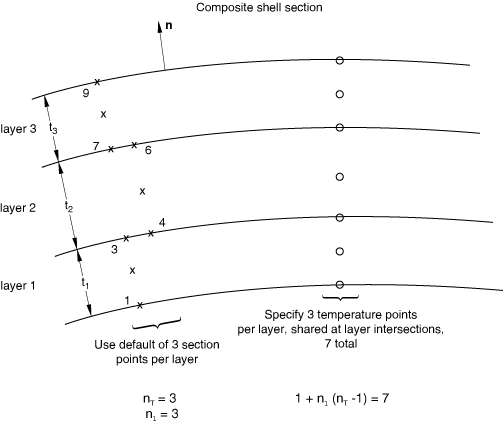
An example of a section with three layers and three section points per layer is shown in
Figure 1.
Figure 1. Example of composite shell section definition.
The material name specified for each layer refers to a material definition (Material Data Definition). The material
behavior can be linear or nonlinear.
The orientation for each layer is specified by either the name of the orientation (Orientations) associated with
the layer or the orientation angle in degrees for the layer. Spatially varying orientation
angles can be specified on a layer using distributions (Distribution Definition). Orientation
angles, , are measured positive counterclockwise around the normal and relative to
the overall section orientation. If either of the two local directions from the overall
section orientation is not in the surface of the shell, is applied after the section orientation has been projected onto the shell
surface. If you do not specify an overall section orientation, is measured relative to the default local shell directions (see Conventions).
You must associate the section properties with a region of your model.
If the orientation definition assigned to a shell section definition is defined with
distributions, spatially varying local coordinate systems are applied to all shell elements
associated with the shell section. A default local coordinate system (as defined by the
distributions) is applied to any shell element that is not specifically included in the
associated distribution.
Unless your model is relatively simple, you will find it increasingly
difficult to define your model using composite shell sections as you increase the number of
layers and as you assign different sections to different regions. It can also be cumbersome
to redefine the sections after you add new layers or remove or reposition existing layers.
To manage a large number of layers in a typical composite model, you might want to use the
composite layup functionality in Abaqus/CAE. For more information, see Composite layups.
where the ELSET parameter refers to
a set of shell elements.
Abaqus/CAE Usage
Abaqus/CAE uses a composite layup or a composite shell section to define the layers of a composite
shell.
Use the following option for a composite layup:
Property module: Create Composite Layup: select Conventional Shell or Continuum Shell as the Element Type: Section integration: During analysis: specify orientations, regions, and materials
Use the following options for a composite shell section:
Property module:
Create Section: select Shell as the section Category and Composite as the section Type: Section integration: During analysisAssignMaterial Orientation: select regions
AssignSection: select regions
Defining the Shell Section Integration
Simpson's rule and Gauss quadrature are provided to calculate the cross-sectional behavior
of a shell. You can specify the number of section points through the thickness of each layer
and the integration method as described below. The default integration method is Simpson's
rule with five points for a homogeneous section and Simpson's rule with three points in each
layer for a composite section.
The three-point Simpson's rule and the two-point Gauss quadrature are exact for linear
problems. The default number of section points should be sufficient for routine
thermal-stress calculations and nonlinear applications (such as predicting the response of
an elastic-plastic shell up to limit load). For more severe thermal shock cases or for more
complex nonlinear calculations involving strain reversals, more section points might be
required; normally no more than nine section points (using Simpson's rule) are required.
Gaussian integration normally requires no more than five section points.
Gauss quadrature provides greater accuracy than Simpson's rule when the same number of
section points are used. Therefore, to obtain comparable levels of accuracy, Gauss
quadrature requires fewer section points than Simpson's rule does and, thus, requires less
computational time and storage space.
Using Simpson's Rule
By default, Simpson's rule will be used for the shell section integration. The default
number of section points is five for a homogeneous section and three in each layer for a
composite section.
Simpson's integration rule should be used if results output on the shell surfaces or
transverse shear stress at the interface between two layers of a composite shell is
required and must be used for heat transfer and coupled temperature-displacement shell
elements.
If you use Gauss quadrature for the shell section integration, the default number of
section points is three for a homogeneous section and two in each layer for a composite
section.
In Gauss quadrature there are no section points on the shell surfaces; therefore, Gauss
quadrature should be used only in cases where results on the shell surfaces are not
required.
Gauss quadrature cannot be used for heat transfer and coupled temperature-displacement
shell elements.
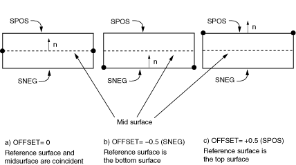
Defining a Shell Offset Value for Conventional Shells
You can define the distance (measured as a fraction of the shell's thickness) from the
shell's midsurface to the reference surface containing the element's nodes (see Defining the Initial Geometry of Conventional Shell Elements). Positive values of the offset are in the positive
normal direction (see About Shell Elements). When the offset is set
equal to 0.5, the top surface of the shell is the reference surface. When the offset is set
equal to −0.5, the bottom surface is the reference surface. The default offset is 0, which
indicates that the middle surface of the shell is the reference surface.
You can specify an offset value that is greater in magnitude than 0.5. However, this
technique should be used with caution in regions of high curvature. The element's area and
all kinematic quantities are calculated relative to the reference surface, which might lead
to a surface area integration error, affecting the stiffness and mass of the shell.
A spatially varying offset can be defined for conventional shells using a distribution
(Distribution Definition). The distribution
used to define the shell offset must have a default value. The default offset is used by any
shell element assigned to the shell section that is not specifically assigned a value in the
distribution.
An offset to the shell's top surface is illustrated in Figure 2.
Figure 2. Schematic of shell offset for an offset value of 0.5.
Input File Usage
Use the following option to specify a value for the shell offset:
The OFFSET parameter accepts a
value, a label (SPOS or
SNEG), or the name of a distribution that is used to
define a spatially varying offset. Specifying SPOS is
equivalent to specifying a value of 0.5; specifying SNEG
is equivalent to specifying a value of −0.5.
Abaqus/CAE Usage
Use the following option for a composite layup:
Property module: composite layup editor: Section integration: During analysis; Offset: choose a reference surface, specify an offset, or select a scalar discrete field
Use the following option for a shell section assignment:
Property module: AssignSection: select regions: Section: select a homogeneous or composite shell section: Definition: select a reference surface, specify an offset, or select a scalar discrete field
Defining a Variable Thickness for Conventional Shells Using Distributions
You can define a spatially varying thickness for conventional shells using a distribution
(Distribution Definition). The thickness of
continuum shell elements is defined by the element geometry.
For composite shells the total thickness is defined by the distribution, and the layer
thicknesses you specify are scaled proportionally such that the sum of the layer thicknesses
is equal to the total thickness (including spatially varying layer thicknesses defined with
a distribution).
The distribution used to define shell thickness must have a default value. The default
thickness is used by any shell element assigned to the shell section that is not
specifically assigned a value in the distribution.
If the shell thickness is defined for a shell section with a distribution, nodal
thicknesses cannot be used for that section definition.
Input File Usage
Use the following option to define a spatially varying thickness:
Use the following option for a conventional shell composite layup:
Property module: composite layup editor: Section integration: During analysis; Shell Parameters: Shell thickness: Element distribution: select an analytical field or an element-based discrete field
Use the following option for a homogeneous shell section:
Property module: shell section editor: Section integration: During analysis; Basic: Shell thickness: Element distribution: select an analytical field or an element-based discrete field
Use the following option for a composite shell section:
Property module: shell section editor: Section integration: During analysis; Advanced: Shell thickness: Element distribution: select an analytical field or an element-based discrete field
Defining a Variable Nodal Thickness for Conventional Shells
You can define a conventional shell with continuously varying thickness by specifying the
thickness of the shell at the nodes. The thickness of continuum shell elements is defined by
the element geometry.
If you indicate that the nodal thicknesses will be specified, for homogeneous shells any
constant shell thickness you specify will be ignored, and the shell thickness will be
interpolated from the nodes. The thickness must be defined at all nodes connected to the
element.
For composite shells the total thickness is interpolated from the nodes, and the layer
thicknesses you specify are scaled proportionally such that the sum of the layer thicknesses
is equal to the total thickness (including spatially varying layer thicknesses defined with
a distribution).
If the shell thickness is defined for a shell section with a distribution, nodal
thicknesses cannot be used for that section definition. However, if nodal thicknesses are
used, you can still use distributions to define spatially varying thicknesses on the layers
of conventional shell elements.
Use the following option for a conventional shell composite layup:
Property module: composite layup editor: Section integration: During analysis; Shell Parameters: Nodal distribution: select an analytical field or a node-based discrete field
Use the following option for a homogeneous shell section:
Property module: shell section editor: Section integration: During analysis; Basic: Nodal distribution: select an analytical field or a node-based discrete field
Use the following option for a composite shell section:
Property module: shell section editor: Section integration: During analysis; Advanced: Nodal distribution: select an analytical field or a node-based discrete field
Defining the Poisson Strain in Shell Elements in the Thickness Direction
Abaqus allows for a possible uniform change in the shell thickness in a geometrically nonlinear
analysis (see Change of Shell Thickness). The
Poisson’s strain can be based on a fixed section Poisson’s ratio, either user specified or
computed by Abaqus based on the elastic portion of the material definition. Alternatively, in Abaqus/Explicit the Poisson strain can be integrated through the section
based on the material response at the individual material points in the section.
By default, Abaqus/Standard computes the Poisson’s strain using a fixed section Poisson’s
ratio of 0.5; Abaqus/Explicit uses the material response to compute the Poisson's strain. See Finite-strain shell element formulation for details
regarding the underlying formulation.
Input File Usage
Use the following option to specify a value for the effective Poisson's ratio:
Use the following option (available only in Abaqus/Explicit) to cause the thickness direction strain under plane stress conditions to be a function
of the membrane strains and the in-plane material properties:
Property module: composite layup editor: Section integration: During analysis; Shell Parameters: Section Poisson's ratio: Use analysis default or Specify value:
Use the following option for a homogeneous or composite shell section:
Property module: shell section editor: Section integration: During analysis; Advanced: Section Poisson's ratio: Use analysis default or Specify value:
You cannot specify a shell thickness direction behavior based on the initial elastic
material definition in Abaqus/CAE.
Defining the Thickness Modulus in Continuum Shell Elements
The thickness modulus is used in computing the stress in the thickness direction (see Thickness Direction Stress in Continuum Shell Elements). By default, Abaqus computes a thickness modulus that is equal to twice the initial in-plane shear modulus
based on the elastic portion of the material definitions in the initial configuration.
Alternatively, you can either provide a value (that is, specify it directly) or let Abaqus compute it as the tensile modulus in the out-of-plane direction based on the elastic
properties in the initial configuration.
If the material properties are unavailable during the preprocessing stage of input; for
example, when the material behavior is defined by the fabric material model or user
subroutine UMAT or VUMAT, you must specify the effective
thickness modulus directly.
Input File Usage
Use the following option to define an effective thickness modulus directly:
THICKNESS MODULUS=ELASTIC
must be used in conjunction with
POISSON=ELASTIC.
Abaqus/CAE Usage
Use the following option for a composite layup:
Property module: composite layup editor: Section integration: During analysis; Shell Parameters: Thickness modulus to specify the thickness properties directly
Use the following option for a homogeneous or composite shell section:
Property module: shell section editor: Section integration: During analysis; Advanced: Thickness modulus to specify the thickness properties directly
You cannot specify a shell thickness direction behavior based on the initial elastic
material definition in Abaqus/CAE.
Defining the Transverse Shear Stiffness
You can provide nondefault values of the transverse shear stiffness. You
must specify the transverse shear stiffness in Abaqus if the section is used with shear flexible shells and the material definitions used in
the shell section do not include linear elasticity, hypoelasticity, or hyperelasticity. See
Shell Section Behavior for more information about transverse
shear stiffness.
If you do not specify the transverse shear stiffness values, Abaqus integrates through the section to determine them. The transverse shear stiffness is
precalculated based on the initial elastic material properties, as defined by the initial
temperature and predefined field variables evaluated at the midpoint of each material layer.
This stiffness is not recalculated during the analysis.
For most shell sections, including layered composite or sandwich shell sections, Abaqus calculates the transverse shear stiffness values required in the element formulation. You
can override these default values. The default shear stiffness values are not calculated in
some cases if estimates of the shear moduli are unavailable during the preprocessing stage
of input; for example, when the material behavior is defined by the fabric material model or
by user subroutines UMAT, UHYPEL, UHYPER, or VUMAT. In such cases (except for
STRI3 elements), you must specify the material
transverse shear modulus (see Defining the Elastic Transverse Shear Modulus) based on which Abaqus calculates the transverse shear stiffness values or define the transverse shear stiffness
for the shell section directly as described below.
You can define additional mass per unit area for conventional shell elements directly in
the section definition. This functionality is similar to the more general functionality of
defining a nonstructural mass contribution (see Nonstructural Mass Definition.) The only
difference between the two definitions is that the nonstructural mass contributes to the
rotary inertia terms about the midsurface while the additional mass defined in the section
definition does not.
Input File Usage
Use the following option to define the density directly:
Property module: composite layup editor: Section integration: During analysis; Shell Parameters: toggle on Density, and enter
Use the following option for a homogeneous or composite shell section:
Property module: shell section editor: Section integration: During analysis; Advanced: toggle on Density, and enter
Specifying Nondefault Hourglass Control Parameters for Reduced-Integration Shell
Elements
You can specify a nondefault hourglass control formulation or scale factors for elements
that use reduced integration. See Section Controls for more
information.
In Abaqus/Standard the nondefault enhanced hourglass control formulation is available only for
S4R and
SC8R elements. When the enhanced hourglass
control formulation is used with composite shells, the average value of the bulk material
properties and the minimum value of the shear material properties over all the layers are
used for computing the hourglass forces and moments.
In Abaqus/Standard you can modify the default values for hourglass control stiffness based on the default
total stiffness approach for elements that use reduced integration and define a scaling
factor for the stiffness associated with the drill degree of freedom (rotation about the
surface normal) for elements that use six degrees of freedom at a node.
The stiffness associated with the drill degree of freedom is the average of the direct
components of the transverse shear stiffness multiplied by a scaling factor. In most cases
the default scaling factor is appropriate for constraining the drill rotation to follow the
in-plane rotation of the element. If an additional scaling factor is defined, the additional
scaling factor should not increase or decrease the drill stiffness by more than a factor of
100.0 for most typical applications. Usually, a scaling factor between 0.1 and 10.0 is
appropriate. Continuum shell elements do not use a drill stiffness; hence, the scale factor
is ignored.
There are no hourglass stiffness factors or scale factors for hourglass stiffness for the
nondefault enhanced hourglass control formulation. You can define the scale factor for the
drill stiffness for the nondefault enhanced hourglass control formulation.
Input File Usage
Use both of the following options to specify a nondefault hourglass control
formulation or scale factors for reduced-integration elements:
Use both of the following options in Abaqus/Standard to modify the default values for hourglass control stiffness based on the default total
stiffness approach for reduced-integration elements and to define a scaling factor for the
stiffness associated with the drill degree of freedom (rotation about the surface normal)
for six degree of freedom elements:
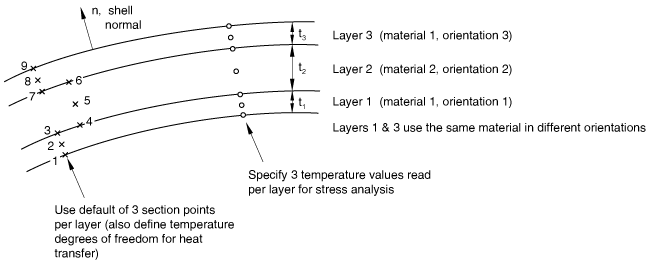
You can specify temperatures and field variables for conventional shell elements by
defining the value at the reference surface of the shell and the gradient through the shell
thickness or by defining the values at equally spaced points through each layer of the
shell's thickness. You can specify a temperature gradient only for elements without
temperature degrees of freedom. The temperatures and field variables for continuum shell
elements are defined at the nodes and then interpolated to the section points.
The actual values of the temperatures and field variables are specified as either
predefined fields or initial conditions (see Predefined Fields or Initial Conditions).
If temperature is to be read as a predefined field from the results file or the output
database file of a previous analysis, the temperature must be defined at equally spaced
points through each layer of the thickness. In addition, the results file must be modified
so that the field variable data are stored in record 201. See Predefined Fields for additional
details.
Defining the Value at the Reference Surface and the Gradient through the
Thickness
You can define the temperature or predefined field by its magnitude on the reference
surface of the shell and the gradient through the thickness. If only one value is given,
the magnitude will be constant through the thickness.
Input File Usage
Use the following option to specify that the temperatures or predefined fields are
defined by a gradient:
Property module: composite layup editor: Section integration: During analysis; Shell Parameters; Temperature variation: Linear through thickness
Use the following option for a homogeneous or composite shell section:
Property module: shell section editor: Section integration: During analysis: Advanced; Temperature variation: Linear through thickness
Only initial temperatures and predefined temperature fields are supported in Abaqus/CAE.
Load module: Create Predefined Field: Step:initial_step or analysis_step: choose Other for the Category and Temperature for the Types for Selected Step
Defining the Values at Equally Spaced Points through the Thickness
Alternatively, you can define the temperature and field variable values at equally spaced
points through the thickness of a shell or of each layer of a composite shell.
For a sequentially coupled thermal-stress analysis in Abaqus/Standard, the number (n) of equally spaced points through the
thickness of a layer is an odd number when temperature values are obtained from the
results file or the output database file generated by a previous Abaqus/Standard heat transfer analysis (since only Simpson's rule can be used for integration through
the section in heat transfer analysis). n may be even or odd if
the values are supplied from some other source. In either case Abaqus/Standard interpolates linearly between the two closest defined temperature points to find the
temperature values at the section points.
The number of predefined field points through each layer, n,
must be the same as the number of integration points used through the same layer in the
analysis from which the temperatures are obtained. This requirement implies that in the
previous analysis each of the layers must have the same number of integration points.
You specify temperature or field variable values, where is the number of layers in the shell section and ( > 1) is the value of n. For =1, you specify temperature or field variable value for a given node or node set.
Input File Usage
Use the following option to specify that the temperatures or predefined fields are
defined at equally spaced points:
Property module: composite layup editor: Section integration: During analysis; Shell Parameters; Temperature variation: Piecewise linear over n values
Use the following option for a homogeneous or composite shell section:
Property module: shell section editor: Section integration: During analysis: Advanced; Temperature variation: Piecewise linear over n values
Only initial temperatures and predefined temperature fields are supported in Abaqus/CAE.
Load module: Create Predefined Field: Step:initial_step or analysis_step: choose Other for the Category and Temperature for the Types for Selected Step
Example
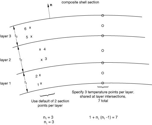
An example of this scheme is illustrated in Figure 3 and Figure 4.
Figure 3. Defining temperature values at n equally spaced points
using Simpson's rule. Figure 4. Defining temperature values at n equally spaced points
using Gauss integration.
The following Abaqus/Standard heat transfer shell section definition corresponds to this example:
This creates degrees of freedom 11–17 in the heat transfer analysis. Temperatures
corresponding to these degrees of freedom are then read into the stress analysis at the
temperature points shown and interpolated to the section points shown.
Defining a Continuous Temperature Field
In Abaqus/Standard if an element with temperature degrees of freedom other than a shell abuts the bottom
surface of a shell element with temperature degrees of freedom, the temperature field is
made continuous when the elements share nodes. If another element with temperature degrees
of freedom abuts the top surface, separate nodes must be used and a linear constraint
equation (Linear Constraint Equations) must be used to
constrain the temperatures to be the same (that is, to give the same value to the top
surface degree of freedom on the shell and degree of freedom 11 on the other element).
For the same reason you must be careful if a different number of temperature points is
used in adjacent shell elements. For compatibility MPCs
(General Multi-Point Constraints) or equation
constraints are also needed in this case.
In Abaqus/Explicit since no thermal MPCs and no thermal equation
constraints are available for degrees of freedom greater than 11, care must be taken when
using a different number of temperature points in adjacent shell elements. This should
usually have a localized effect on the temperature distribution, but it might affect the
overall solution for the cases in which the temperature gradient through the thickness is
significant.
In both Abaqus/Standard and Abaqus/Explicit be careful in the models in which the shell's normals are reversed. In this case the
temperature at the bottom of the shell becomes the temperature at the top of the adjacent
shell. This might have a small impact on the overall solution for the cases in which the
thermal gradient through the thickness is negligible and the temperature variation is
mainly in plane. However, if the temperature gradient through the thickness is
significant, it might lead to incorrect results.
Output
In an Abaqus/Standard stress analysis, temperature output at the section points can be obtained using the
element variable TEMP.
If the temperature values were specified at equally spaced points through the thickness,
output at the temperature points can be obtained in an Abaqus/Standard stress analysis, as in a heat transfer analysis, by using the nodal variable
NTxx. This
nodal output variable is also available in Abaqus/Explicit for coupled temperature-displacement analyses. The nodal variable
NTxx should not
be used for output at the temperature points with the default gradient method. In this case
output variable NT should be requested;
NT11 (the reference temperature value) and
NT12 (the temperature gradient) will be
output automatically. For continuum shell elements, there is only
NT11; all other
NTxx are
irrelevant.
Other output variables that are relevant for shells are listed in each of the library
sections describing the specific shell elements. For example, stresses, strains, section
forces and moments, average section stresses, section strains, etc. can be output. The
section moments are calculated relative to the reference surface.