Mode-Based Steady-State Dynamic Analysis

Introduction

Steady-state dynamic analysis provides the steady-state amplitude and phase of the response of a system due to harmonic excitation at a given frequency. Usually such analysis is done as a frequency sweep by applying the loading at a series of different frequencies and recording the response; in Abaqus/Standard the steady-state dynamic analysis procedure is used to conduct the frequency sweep.

In a mode-based steady-state dynamic analysis, the response is based on modal superposition techniques; the modes of the system must first be extracted using the eigenfrequency extraction procedure. The modes will include eigenmodes and, if activated in the eigenfrequency extraction step, residual modes. The number of modes extracted must be sufficient to model the dynamic response of the system adequately, which is a matter of judgment on your part.

When defining a mode-based steady-state dynamic step, you specify the frequency ranges of interest and the number of frequencies at which results are required in each range (including the bounding frequencies of the range). In addition, you can specify the type of frequency spacing (linear or logarithmic) to be used, as described below (Selecting the Frequency Spacing). Logarithmic frequency spacing is the default. Frequencies are given in cycles/time.

These frequency points for which results are required can be spaced equally along the frequency axis (on a linear or a logarithmic scale), or they can be biased toward the ends of the user-defined frequency range by introducing a bias parameter (see The Bias Parameter below).

While the response in this procedure is for linear vibrations, the prior response can be nonlinear. Initial stress effects (stress stiffening) will be included in the steady-state dynamics response if nonlinear geometric effects (General and Perturbation Procedures) were included in any general analysis step prior to the eigenfrequency extraction step preceding the steady-state dynamic procedure.

Input File Usage

STEADY STATE DYNAMICS

The DIRECT and SUBSPACE PROJECTION parameters must be omitted from the STEADY STATE DYNAMICS option to conduct a mode-based steady-state dynamic analysis.

Abaqus/CAE Usage

Step module: Create Step: Linear perturbation: Steady-state 
dynamics, Modal

Selecting the Type of Frequency Interval for Which Output Is Requested

Three types of frequency intervals are permitted for output from a mode-based steady-state dynamic step.

Specifying the Frequency Ranges by Using the System's Eigenfrequencies

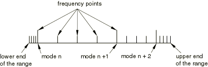
By default, the eigenfrequency type of frequency interval is used; in this case the following intervals exist in each frequency range:

First interval: extends from the lower limit of the frequency range given to the first eigenfrequency in the range.
Intermediate intervals: extend from eigenfrequency to eigenfrequency.
Last interval: extends from the highest eigenfrequency in the range to the upper limit of the frequency range.

For each of these intervals the frequencies at which results are calculated are determined using the user-defined number of points (which includes the bounding frequencies for the interval) and the optional bias function (which is discussed below and allows the sampling points on the frequency scale to be spaced closer together at eigenfrequencies in the frequency range). Thus, detailed definition of the response close to resonance frequencies is allowed. Figure 1 illustrates the division of the frequency range for 5 calculation points and a bias parameter equal to 1.

Input File Usage

STEADY STATE DYNAMICS, INTERVAL=EIGENFREQUENCY

Abaqus/CAE Usage

Step module: Create Step: Linear perturbation: Steady-state 
dynamics, Modal: Use eigenfrequencies to subdivide each frequency range

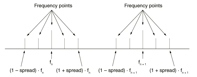
Specifying the Frequency Ranges by the Frequency Spread

If the spread type of frequency interval is selected, intervals exist around each eigenfrequency in the frequency range. For each of the intervals the equally spaced frequencies at which results are calculated are determined using the user-defined number of points (which includes the bounding frequencies for the interval). The minimum number of frequency points is 3. If the user-defined value is less than 3 (or omitted), the default value of 3 points is assumed. Figure 2 illustrates the division of the frequency range for 5 calculation points.

The bias parameter is not supported with the spread type of frequency interval.

Input File Usage

STEADY STATE DYNAMICS, INTERVAL=SPREAD
lwr_freq, upr_freq, numpts, bias_param, freq_scale_factor, spread

Abaqus/CAE Usage

You cannot specify frequency ranges by frequency spread in Abaqus/CAE.

Specifying the Frequency Ranges Directly

If the alternative range type of frequency interval is chosen, there is only one interval in the specified frequency range spanning from the lower to the upper limit of the range. This interval is divided using the user-defined number of points and the optional bias function, which can be used to space the sampling frequency points closer to the range limits. For the range type of frequency interval, the peak responses around the system's eigenfrequencies might be missed since the sampling frequencies at which output will be reported will not be biased toward the eigenfrequencies.

Input File Usage

STEADY STATE DYNAMICS, INTERVAL=RANGE

Abaqus/CAE Usage

Step module: Create Step: Linear perturbation: Steady-state 
dynamics, Modal: toggle off Use eigenfrequencies to subdivide each frequency range

Selecting the Frequency Spacing

Two types of frequency spacing are permitted for a mode-based steady-state dynamic step. For the logarithmic frequency spacing (the default), the specified frequency ranges of interest are divided using a logarithmic scale. Alternatively, a linear frequency spacing can be used if a linear scale is desired.

Input File Usage

Use either of the following options:

STEADY STATE DYNAMICS, FREQUENCY SCALE=LOGARITHMIC
STEADY STATE DYNAMICS, FREQUENCY SCALE=LINEAR

Abaqus/CAE Usage

Step module: Create Step: Linear perturbation: Steady-state dynamics, Modal: Scale: Logarithmic or Linear

Requesting Multiple Frequency Ranges

You can request multiple frequency ranges or multiple single frequency points for a mode-based steady-state dynamic step.

Input File Usage

STEADY STATE DYNAMICS
lwr_freq1, upr_freq1, numpts1, bias_param1, freq_scale_factor1
lwr_freq2, upr_freq2, numpts2, bias_param2, freq_scale_factor2
...
single_freq1
single_freq2
...

Repeat the data lines as often as necessary.

Abaqus/CAE Usage

Step module: Create Step: Linear perturbation: Steady-state dynamics, Modal: Data: enter data in table, and add rows as necessary

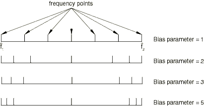
The Bias Parameter

The bias parameter can be used to provide closer spacing of the results points either toward the middle or toward the ends of each frequency interval. Figure 3 shows a few examples of the effect of the bias parameter on the frequency spacing.

The bias formula used to calculate the frequency at which results are presented is as follows:

{\hat{f}}_{k} = \frac{1}{2} ({\hat{f}}_{1} + {\hat{f}}_{2}) + \frac{1}{2} ({\hat{f}}_{2} - {\hat{f}}_{1}) {| y |}^{1 / p} sign (y),

where

y: $ = - 1 + 2 (k - 1) / (n - 1)$ ;
n: is the number of frequency points at which results are to be given within a frequency interval (discussed above);
k: is one such frequency point ( $k = 1, 2, \dots, n$ );
${\hat{f}}_{1}$: is the lower limit of the frequency interval;
${\hat{f}}_{2}$: is the upper limit of the frequency interval;
${\hat{f}}_{k}$: is the frequency at which the kth results are given;
p: is the bias parameter value; and
$\hat{f}$: is the frequency or the logarithm of the frequency, depending on the value used for the frequency scale parameter.

A bias parameter, p, that is greater than 1.0 provides closer spacing of the results points toward the ends of the frequency interval, while values of p that are less than 1.0 provide closer spacing toward the middle of the frequency interval. The default bias parameter is 3.0 for an eigenfrequency interval and 1.0 for a range frequency interval.

The Frequency Scale Factor

The frequency scale factor can be used to scale frequency points. All the frequency points, except the lower and upper limit of the frequency range, are multiplied by this factor. This scale factor can be used only when the frequency interval is specified by using the system's eigenfrequencies (see Specifying the Frequency Ranges by Using the System's Eigenfrequencies above).

Selecting the Modes and Specifying Damping

You can select the modes to be used in modal superposition and specify damping values for all selected modes.

Selecting the Modes

You can select modes by specifying the mode numbers individually, by requesting that Abaqus/Standard generate the mode numbers automatically, or by requesting the modes that belong to specified frequency ranges. If you do not select the modes, all modes extracted in the prior eigenfrequency extraction step, including residual modes if they were activated, are used in the modal superposition.

Input File Usage

Use one of the following options to select the modes by specifying mode numbers:

SELECT EIGENMODES, DEFINITION=MODE NUMBERS
SELECT EIGENMODES, GENERATE, DEFINITION=MODE NUMBERS

Use the following option to select the modes by specifying a frequency range:

SELECT EIGENMODES, DEFINITION=FREQUENCY RANGE

Abaqus/CAE Usage

You cannot select the modes in Abaqus/CAE; all modes extracted are used in the modal superposition.

Specifying Modal Damping

Damping is almost always specified for a steady-state analysis (see Material Damping). If damping is absent, the response of a structure will be unbounded if the forcing frequency is equal to an eigenfrequency of the structure. To get quantitatively accurate results, especially near natural frequencies, accurate specification of damping properties is essential. The various damping options available are discussed in Material Damping. 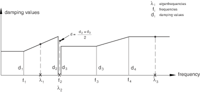You can define a damping coefficient for all or some of the modes used in the response calculation. The damping coefficient can be given for a specified mode number or for a specified frequency range. When damping is defined by specifying a frequency range, the damping coefficient for a mode is interpolated linearly between the specified frequencies. The frequency range can be discontinuous; the average damping value will be applied for an eigenfrequency at a discontinuity. The damping coefficients are assumed to be constant outside the range of specified frequencies.

Input File Usage

Use the following option to define damping by specifying mode numbers:

MODAL DAMPING, DEFINITION=MODE NUMBERS

Use the following option to define damping by specifying a frequency range:

MODAL DAMPING, DEFINITION=FREQUENCY RANGE

Abaqus/CAE Usage

Use the following input to define damping by specifying mode numbers:

Step module: Create Step: Linear perturbation:
Steady-state dynamics, Modal: Damping

Example of Specifying Damping

Figure 4 illustrates how the damping coefficients at different eigenfrequencies are determined for the following input:

MODAL DAMPING, DEFINITION=FREQUENCY RANGE
 $f_{1}, d_{1}$ 
 $f_{2}, d_{2}$ 
 $f_{2}, d_{3}$ 
 $f_{3}, d_{3}$ 
 $f_{4}, d_{4}$

Rules for Selecting Modes and Specifying Damping Coefficients

The following rules apply for selecting modes and specifying modal damping coefficients:

No modal damping is included by default.
Mode selection and modal damping must be specified in the same way, using either mode numbers or a frequency range.
If you do not select any modes, all modes extracted in the prior frequency analysis, including residual modes if they were activated, will be used in the superposition.
If you do not specify damping coefficients for modes that you have selected, zero damping values will be used for these modes.
Damping is applied only to the modes that are selected.
Damping coefficients for selected modes that are beyond the specified frequency range are constant and equal to the damping coefficient specified for the first or the last frequency (depending which one is closer). This is consistent with the way Abaqus interprets amplitude definitions.

Specifying Global Damping

For convenience you can specify constant global damping factors for all selected eigenmodes for mass and stiffness proportional viscous factors, as well as stiffness proportional structural damping. For further details, see Damping in Dynamic Analysis.

Input File Usage

Use the following option to define damping by global factors:

GLOBAL DAMPING, ALPHA=factor, BETA=factor, STRUCTURAL=factor

Abaqus/CAE Usage

Defining damping by global factors is not supported in Abaqus/CAE.

Material Damping

Structural and viscous material damping (see Material Damping) is taken into account in a SIM-based steady-state dynamic analysis. Since the projection of damping onto the mode shapes is performed only one time during the frequency extraction step, significant performance advantages can be achieved by using the SIM-based steady-state dynamic procedure (see Using the SIM Architecture for Modal Superposition Dynamic Analyses).

If the damping operators depend on frequency, they will be evaluated at the frequency specified for property evaluation during the frequency extraction procedure.

You can deactivate the structural or viscous damping in a mode-based steady-state dynamic procedure if desired.

Input File Usage

Use the following option to deactivate structural and viscous damping in a specific steady-state dynamic step:

DAMPING CONTROLS, STRUCTURAL=NONE, VISCOUS=NONE

Abaqus/CAE Usage

Damping controls are not supported in Abaqus/CAE.

Initial Conditions

The base state is the current state of the model at the end of the last general analysis step before the steady-state dynamic step. If the first step of an analysis is a perturbation step, the base state is determined from the initial conditions (Initial Conditions). Initial condition definitions that directly define solution variables, such as velocity, cannot be used in a steady-state dynamic analysis.

Boundary Conditions

In a mode-based steady-state dynamic analysis, both the real and imaginary parts of any degree of freedom are either restrained or unrestrained; it is physically impossible to have one part restrained and the other part unrestrained. Abaqus/Standard will automatically restrain both the real and imaginary parts of a degree of freedom even if only one part is restrained.

Base Motion

It is not possible to prescribe nonzero displacements and rotations directly as boundary conditions (Boundary Conditions) in mode-based dynamic response procedures. Therefore, in a mode-based steady-state dynamic analysis, the motion of nodes can be specified only as base motion; nonzero displacement or acceleration history definitions given as boundary conditions are ignored, and any changes in the support conditions from the eigenfrequency extraction step are flagged as errors. The method for prescribing base motion in modal superposition procedures is described in Transient Modal Dynamic Analysis.

Base motions can be defined by a displacement, a velocity, or an acceleration history. For an acoustic pressure, the displacement is used to describe an acoustic pressure history. If the prescribed excitation record is given in the form of a displacement or velocity history, Abaqus/Standard differentiates it to obtain the acceleration history. The default is to give an acceleration history for mechanical degrees of freedom and to give a displacement for an acoustic pressure.

When secondary bases are used, low frequency eigenmodes will be extracted for each “big” mass applied in the model. Use care when choosing the frequency lower limit range in such cases. The “big” mass modes are important in the modal superposition; however, the response at zero or arbitrarily low frequency level should not be requested since it forces Abaqus/Standard to calculate responses at frequencies between these “big” mass eigenfrequencies, which is not desirable.

Frequency-Dependent Base Motion

An amplitude definition can be used to specify the amplitude of a base motion as a function of frequency (Amplitude Curves).

Input File Usage

Use both of the following options:

AMPLITUDE, NAME=name
BASE MOTION, REAL or IMAGINARY, AMPLITUDE=name

Abaqus/CAE Usage

Load module; Create Boundary Condition; Step: step_name; Category: Mechanical; Types for Selected Step: Displacement base motion or Velocity base motion or Acceleration base motion; Basic tabbed page: Degree-of-freedom: U1, U2, U3, UR1, UR2, or UR3; Amplitude: name

Loads

The following loads can be prescribed in a mode-based steady-state dynamic analysis, as described in Concentrated Loads:

Concentrated nodal forces can be applied to the displacement degrees of freedom (1–6).
Distributed pressure forces or body forces can be applied; the distributed load types available with particular elements are described in Abaqus Elements Guide.

These loads are assumed to vary sinusoidally with time over a user-specified range of frequencies. Loads are given in terms of their real and imaginary components.

Fluid flux loading cannot be used in a steady-state dynamic analysis.

Input File Usage

Use either of the following input lines to define the real (in-phase) part of the load:

CLOAD or DLOAD
CLOAD or DLOAD, REAL

Use the following input line to define the imaginary (out-of-phase) part of the load:

CLOAD or DLOAD, IMAGINARY

Abaqus/CAE Usage

Load module: load editor: real (in-phase) part + imaginary (out-of-phase) parti

Frequency-Dependent Loading

An amplitude definition can be used to specify the amplitude of a load as a function of frequency (Amplitude Curves).

Input File Usage

Use both of the following options:

AMPLITUDE, NAME=name
CLOAD or DLOAD, REAL or IMAGINARY, AMPLITUDE=name

Abaqus/CAE Usage

Load or Interaction module: Create Amplitude: Name:name

Load module: load editor: real (in-phase) part + imaginary (out-of-phase) parti: Amplitude:name

Predefined Fields

Predefined temperature fields are not allowed in mode-based steady-state dynamic analysis. Other predefined fields are ignored.

Material Options

As in any dynamic analysis procedure, mass or density (Density) must be assigned to some regions of any separate parts of the model where dynamic response is required. The following material properties are not active during mode-based steady-state dynamic analyses: plasticity and other inelastic effects, viscoelastic effects, thermal properties, mass diffusion properties, electrical properties (except for the electrical potential, $ϕ$ , in piezoelectric analysis), and pore fluid flow properties—see General and Perturbation Procedures.

Elements

Any of the following elements available in Abaqus/Standard can be used in a steady-state dynamics procedure:

stress/displacement elements (other than generalized axisymmetric elements with twist);
acoustic elements;
piezoelectric elements; or
hydrostatic fluid elements.

See Choosing the Appropriate Element for an Analysis Type.

Output

In mode-based steady-state dynamic analysis the value of an output variable such as strain (E) or stress (S) is a complex number with real and imaginary components. In the case of data file output, the first printed line gives the real components while the second lists the imaginary components. Results and data file output variables are also provided to obtain the magnitude and phase of many variables (see Abaqus/Standard Output Variable Identifiers). In this case the first printed line in the data file gives the magnitude while the second gives the phase angle.

In steady-state dynamic analysis procedures, you can request output for load cases to store only relevant results for each load case. This can reduce the size of the output database.

For more information, see Variables Available for Mode-Based Steady-State Dynamic Analysis.

Total Energy Output

The energy variables that can be written to the output database are defined in Total Energy Output Quantities. In modal steady-state dynamics analysis the following energy output variables are available: ALLWK, ALLKE, ALLKEA, ALLKEP, ALLSE, ALLSEA, ALLSEP, ALLVD, ALLVDE, ALLVDG, ALLVDM, ALLHD, ALLHDE, ALLHDG, ALLHDM, EFLOW, PFLOW, RADEN, and RADPOW.

The following energies are not available as element set quantities: ALLWK, ALLVDM, and ALLHDM.

Energy dissipation due to viscous and structural damping is represented by the following output variables: ALLVD, ALLVDE, ALLVDG, ALLVDM, ALLHD, ALLHDE, ALLHDG, and ALLHDM. In addition, you can examine energy loss due to material, global, and modal damping as represented by the following output variables: ALLVDE and ALLHDE for material damping, ALLVDG and ALLHDG for global damping, and ALLVDM and ALLHDM for modal damping.

Input File Usage

ENERGY OUTPUT
list of output variables

Abaqus/CAE Usage

Step module: history output request editor: Select from list below

Energy and Power Flow

Modal steady-state dynamic analysis supports the computation of the energy and power flow from/into a portion of the model (represented by an element set) through a boundary (represented by a node set). Energy flow is represented by output variable EFLOW, while power flow is given by output variable PFLOW.

Input File Usage

ENERGY OUTPUT, ELSET=elset_name, NSET=nset_name
EFLOW, PFLOW

Abaqus/CAE Usage

Output for energy and power flow is not supported in Abaqus/CAE.

Radiated Energy and Power

Modal steady-state dynamic analysis supports the computation of the radiated acoustic energy and power from/into an acoustic cavity (represented by an element set of acoustic elements) through a portion of the structural-acoustic interface (represented by a node set containing nodes of structural elements). Radiated energy is represented by output variable RADEN, while radiated power is given by output variable RADPOW. The element set representing the acoustic cavity can consist of just one element in that acoustic cavity. The contribution of the other acoustic elements belonging to the same cavity is computed automatically.

Input File Usage

ENERGY OUTPUT, ELSET=elset_name, NSET=nset_name
RADEN, RADPOW

Abaqus/CAE Usage

Output for radiated energy and power is not supported in Abaqus/CAE.

Whole Element Energy Output

The whole element energy variables that can be written to the output database are defined in Whole Element Energy Density Variables. Modal steady-state dynamic analysis supports the computation of mean values of kinetic and potential energies in the finite elements (ELKE and ELSE) as well as the total energy loss for the period due to viscous and structural damping (ELVD, ELVDE, ELVDG, ELHD, ELHDE, and ELHDG).

Computation of the amplitude and peak values of the kinetic and potential energies is provided (ELKEA, ELKEP, ELSEA, and ELSEP). In addition, computation of various energy densities is supported (EKEDEN, EKEDENA, EKEDENP, ESEDEN, ESEDENA, ESEDENP, EVDDEN, EVDDENE, EVDDENG, EHDDEN, EHDDENE, and EHDDENG).

Acoustic Contribution Factors

Computation of the acoustic contribution factors helps you determine the major noise sources. The procedure for computing the acoustic contribution factors is based on the modal analysis formulation of acoustic-structural problems with uncoupled modes. For more information, see Acoustic Contribution Factors in Mode-Based and Subspace-Based Steady-State Dynamic Analyses.

Variables Available for Mode-Based Steady-State Dynamic Analysis

The following variables are provided specifically for steady-state dynamic analysis:

Element integration point variables:

PHS: Magnitude and phase angle of all stress components.
PHE: Magnitude and phase angle of all strain components.
PHEPG: Magnitude and phase angles of the electrical potential gradient vector.
PHEFL: Magnitude and phase angles of the electrical flux vector.
PHMFL: Magnitude and phase angle of the mass flow rate in fluid link elements.
PHMFT: Magnitude and phase angle of the total mass flow in fluid link elements.

For connector elements, the following element output variables are available:

PHCTF: Magnitude and phase angle of connector total forces.
PHCEF: Magnitude and phase angle of connector elastic forces.
PHCVF: Magnitude and phase angle of connector viscous forces.
PHCRF: Magnitude and phase angle of connector reaction forces.
PHCSF: Magnitude and phase angle of connector friction forces.
PHCU: Magnitude and phase angle of connector relative displacements.
PHCCU: Magnitude and phase angle of connector constitutive displacements.

Nodal variables:

PU: Magnitude and phase angle of all displacement/rotation components at a node.
PPOR: Magnitude and phase angle of the fluid or acoustic pressure at a node.
PHPOT: Magnitude and phase angle of the electrical potential at a node.
PRF: Magnitude and phase angle of all reaction forces/moments at a node.
PHCHG: Magnitude and phase angle of the reactive charge at a node.

The following energy output variables are available in a mode-based steady-state dynamic analysis:

Total energy output variables:

ALLKE: Kinetic energy. In steady-state dynamic analysis this is the cyclic mean value.
ALLKEA: Kinetic energy amplitude.
ALLKEP: Kinetic energy peak value.
ALLSE: Recoverable strain energy. In steady-state dynamic analysis this is the cyclic mean value.
ALLSEA: Recoverable strain energy amplitude.
ALLSEP: Recoverable strain energy peak value.
ALLVD: Energy dissipated by viscous effects including viscous regularization (except for cohesive elements and cohesive contact), not inclusive of energy dissipated by automatic stabilization and viscoelasticity. If this variable is requested for the whole model, it includes energy loss due to the material, global, and modal damping. If this variable is requested for a part of the model, energy loss due to the modal damping is not included.
ALLVDE: Energy dissipated by viscous effects due to the material damping.
ALLVDG: Energy dissipated by viscous effects due to the global damping.
ALLVDM: Energy dissipated by viscous effects due to the modal damping. This variable is available for the whole model.
ALLHD: Energy dissipated due to the structural damping. If this variable is requested for the whole model, it includes energy loss due to the material, global, and modal damping. If this variable is requested for a part of the model, energy loss due to the modal damping is not included.
ALLHDE: Energy dissipated due to the material structural damping.
ALLHDG: Energy dissipated due to the global structural damping.
ALLHDM: Energy dissipated due to the modal structural damping. This variable is available for the whole model.
ALLWK: External work. (Available only for the whole model.)
EFLOW: Energy flow from a given portion of the model through the given boundary.
PFLOW: Power flow from a given portion of the model through the given boundary.
RADEN: Radiated energy from/into a given acoustic cavity through the given boundary.
RADPOW: Radiated power from/into a given acoustic cavity through the given boundary.

Whole element energy variables:

ELKE: Total kinetic energy in the element. In steady-state dynamic analysis this is the cyclic mean value.
ELKEA: Total kinetic energy amplitude in the element.
ELKEP: Total kinetic energy peak value in the element.
ELSE: Total elastic strain energy in the element. When the Mullins effect is modeled with hyperelastic materials, this quantity represents only the recoverable part of energy in the element. In steady-state dynamic analysis this is the cyclic mean value.
ELSEA: Total elastic strain energy amplitude in the element.
ELSEP: Total elastic strain energy peak value in the element.
ELVD: Total energy dissipated in the element by viscous effects, not including energy dissipated by static stabilization or viscoelasticity.
ELVDE: Total energy dissipated in the element by viscous effects due to the material damping.
ELVDG: Total energy dissipated in the element by viscous effects due to the global damping.
ELHD: Total energy dissipated in the element due to structural damping. This variable includes energy loss due to the material and global structural damping.
ELHDE: Total energy dissipated in the element due to the material structural damping.
ELHDG: Total energy dissipated in the element due to the global structural damping.

Whole element energy density variables:

EKEDEN: Kinetic energy density in the element. In steady-state dynamic analysis this is the cyclic mean value.
EKEDENA: Kinetic energy density amplitude in the element.
EKEDENP: Kinetic energy density peak value in the element.
ESEDEN: Total elastic strain energy density in the element. When the Mullins effect is modeled with hyperelastic materials, this quantity represents only the recoverable part of energy density in the element. This variable is not available in eigenvalue extraction procedures. In steady-state dynamic analysis this is the cyclic mean value.
ESEDENA: Total elastic strain energy density amplitude in the element.
ESEDENP: Total elastic strain energy density peak value in the element.
EVDDEN: Total energy dissipated per unit volume in the element by viscous effects, not inclusive of energy dissipated through static stabilization or viscoelasticity.
EVDDENE: Total energy dissipated per unit volume in the element by viscous effects due to the material damping.
EVDDENG: Total energy dissipated per unit volume in the element by viscous effects due to the global damping.
EHDDEN: Total energy dissipated per unit volume in the element due to structural damping. This variable includes energy loss due to the material and global structural damping.
EHDDENE: Total energy dissipated per unit volume in the element due to the material structural damping.
EHDDENG: Total energy dissipated per unit volume in the element due to the global structural damping.

The standard output variables U, V, A, and the variable PU listed above correspond to motions relative to the motion of the primary base in a mode-based analysis. Total values, which include the motion of the primary base, are also available:

TU: Magnitude of all components of total displacement/rotation at a node.
TV: Magnitude of all components of total velocity at a node.
TA: Magnitude of all components of total acceleration at a node.
PTU: Magnitude and phase angle of all total displacement/rotation components at a node.

The following modal variables are also available for mode-based steady-state dynamic analysis and can be output to the data, results, and/or output database files (see Output to the Data and Results Files and Output to the Output Database):

GU: Generalized displacements for all modes.
GV: Generalized velocities for all modes.
GA: Generalized accelerations for all modes.
GPU: Phase angle of generalized displacements for all modes.
GPV: Phase angle of generalized velocities for all modes.
GPA: Phase angle of generalized acceleration for all modes.
SNE: Elastic strain energy for the entire model per mode.
KE: Kinetic energy for the entire model per mode.
T: External work for the entire model per mode.
BM: Base motion.

Whole model variables such as ALLIE (total strain energy) are available for mode-based steady-state dynamics as output to the data, results, and/or output database files (see Output to the Data and Results Files).

Input File Template

HEADING
…
AMPLITUDE, NAME=loadamp
Data lines to define an amplitude curve as a function of frequency (cycles/time)
AMPLITUDE, NAME=base
Data lines to define an amplitude curve to be used to prescribe base motion
**
STEP, NLGEOM
Include the NLGEOM parameter so that stress stiffening effects will
be included in the steady-state dynamics step
STATIC
**Any general analysis procedure can be used to preload the structure
…
CLOAD and/or DLOAD
Data lines to prescribe preloads
TEMPERATURE and/or FIELD
Data lines to define values of predefined fields for preloading the structure
BOUNDARY
Data lines to specify boundary conditions to preload the structure
END STEP
**
STEP
FREQUENCY
Data line to control eigenvalue extraction
BOUNDARY
Data lines to assign degrees of freedom to the primary base
BOUNDARY, BASE NAME=base2
Data lines to assign degrees of freedom to a secondary base
END STEP
**
STEP
STEADY STATE DYNAMICS
Data lines to specify frequency ranges and bias parameters
SELECT EIGENMODES
Data lines to define the applicable mode ranges
ACOUSTIC CONTRIBUTION
MODAL DAMPING
Data lines to define the modal damping factors
BASE MOTION, DOF=dof, AMPLITUDE=base
BASE MOTION, DOF=dof, AMPLITUDE=base, BASE NAME=base2
CLOAD and/or DLOAD, AMPLITUDE=loadamp
Data lines to specify sinusoidally varying, frequency-dependent loads
…
END STEP