Low-Cycle Fatigue Analysis Using the Direct Cyclic Approach

The direct cyclic analysis capability in Abaqus/Standard provides a computationally effective modeling technique to obtain the stabilized response of a structure subjected to periodic loading and is ideally suited to perform low-cycle fatigue calculations on a large structure. The capability uses a combination of Fourier series and time integration of the nonlinear material behavior to obtain the stabilized response of the structure directly. The theory and algorithm to obtain a stabilized response using the direct cyclic approach are described in detail in Direct cyclic algorithm.

The direct cyclic low-cycle fatigue procedure models the progressive damage and failure both in bulk materials (such as in solder joints in an electronic chip packaging or intra-laminar crack growth in laminated composites) and at material interfaces (such as delamination in laminated composites). 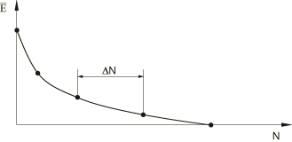The former can be based on either a continuum damage mechanics approach or the principles of linear elastic fracture mechanics with the extended finite element method. The response is obtained by evaluating the behavior of the structure at discrete points along the loading history (see Figure 1). The solution at each of these points is used to predict the degradation and evolution of material properties that will take place during the next increment, which spans a number of load cycles, $\mathrm{\Delta }N$ . The degraded material properties are then used to compute the solution at the next increment in the load history. Therefore, the crack/damage growth rate is updated continually throughout the analysis.

Figure 1. Elastic stiffness degradation as a function of the cycle number.

The elastic material stiffness at a material point remains constant and contact conditions remain unchanged when the stabilized solution is computed at a given point in the loading history. Each of the solutions along the loading history represents the stabilized response of the structure subjected to the applied period loads, with a level of material damage at each point in the structure computed from the previous solution. This process is repeated up to a point in the loading history at which a fatigue life assessment can be made.

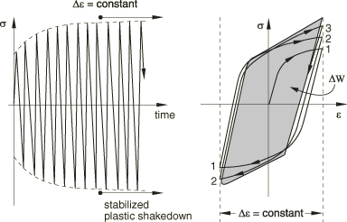
In bulk material, there are two approaches to modeling the progressive damage and failure. One approach is based on continuum damage mechanics. This approach is more appropriate for ductile material, in which the cyclic loading leads to stress reversals and the accumulation of plastic strains, which in turn cause the initiation and propagation of cracks. The damage initiation and evolution are characterized by the stabilized accumulated inelastic hysteresis strain energy per cycle as illustrated in Figure 2. The other approach is based on the principles of linear elastic fracture mechanics with the extended finite element method. This approach is more appropriate for brittle material or material with small scale yielding, in which the cyclic loading leads to material strength degradation causing fatigue crack growth along an arbitrary path. The onset and growth of the crack are characterized by the relative fracture energy release rate at the crack tip based on the Paris law (Paris, 1961).

Figure 2. Plastic shakedown in a direct cyclic analysis.

At interfaces of laminated composites, the cyclic loading leads to interface strength degradation causing fatigue delamination growth. The onset and growth of delamination are also characterized by the relative fracture energy release rate at the crack tip based on the Paris law (Paris, 1961).

Both the progressive damage mechanism in the bulk material and the progressive delamination growth mechanism at interfaces can be considered simultaneously, with the failure occurring first at the weakest link in a model.

Defining a low-cycle fatigue analysis using the direct cyclic approach is similar to defining a direct cyclic analysis. See Direct Cyclic Analysis for details on how to specify the number of Fourier terms, number of iterations, and the increment sizes. You specify the maximum numbers of cycles, $N_{max}$ , when you define the low-cycle fatigue analysis step.

DIRECT CYCLIC, FATIGUE
first data line
 , , $N_{max}$

Step module: Create Step: General: Direct cyclic; Fatigue: Include low-cycle fatigue analysis, Maximum number of cycles: Value: $N_{max}$

A low-cycle fatigue step using the direct cyclic approach can be the only step in an analysis, can follow a general or linear perturbation step, or can be followed by a general or linear perturbation step. Multiple low-cycle fatigue analysis steps can be included in a single analysis. In such a case the Fourier series coefficients obtained in the previous step can be used as starting values in the current step. By default, the Fourier coefficients are reset to zero, thus allowing application of cyclic loading conditions that are very different from those defined in the previous low-cycle fatigue step.

As in a direct cyclic analysis, you can specify that a low-cycle fatigue step in a restart analysis should use the Fourier coefficients from the previous step, thus allowing continuation of an analysis to simulate more loading cycles. In a low-cycle fatigue analysis, a restart file is written at the end of the stabilized cycle. Consequently, a restart analysis that is a continuation of a previous low-cycle fatigue analysis will start with a new loading cycle at $t=0$ (see Restarting an Analysis).

DIRECT CYCLIC,  FATIGUE, CONTINUE=YES

DIRECT CYCLIC,  FATIGUE, CONTINUE=NO (default)

Step module: Create Step: General: Direct cyclic; Basic: Use displacement Fourier coefficients from previous direct cyclic step; Fatigue: Include low-cycle fatigue analysis

Step module: Create Step: General: Direct cyclic; Fatigue: Include low-cycle fatigue analysis

Damage initiation refers to the beginning of degradation of the response of a material point. In a low-cycle fatigue analysis the damage initiation criterion is characterized by the accumulated inelastic hysteresis energy per cycle, $\mathrm{\Delta }w$ . $\mathrm{\Delta }w$ and material constants are used to determine the number of the cycle in which damage is initiated, $N_0$ . At the end of a stabilized loading cycle, $N$ , Abaqus/Standard checks to see if the damage initiation criterion $N>N_0$ is satisfied in any material point; material stiffness at a material point will not be degraded unless this criterion is satisfied. The calculations and output associated with damage initiation are discussed in detail in Damage Initiation for Ductile Materials in Low-Cycle Fatigue.

Once the damage initiation criterion is satisfied at a material point, the damage state is calculated and updated based on the inelastic hysteresis energy for the stabilized cycle. Abaqus/Standard assumes that the degradation of the elastic stiffness can be modeled using the scalar damage variable, $D$ . The rate of the damage in a material point per cycle, $\frac{dD}{dN}$ , is calculated based on the accumulated inelastic hysteresis energy, the characteristic length associated with an integration point, and material constants. For details, see Damage Evolution for Ductile Materials in Low-Cycle Fatigue.

Typically, a material has completely lost its load-carrying capacity when $D=1$ . You can remove an element from the mesh if all the section points at all integration locations of the element have lost their load-carrying capability.

If the damage initiation criterion is satisfied in any material point at the end of a stabilized cycle, $N$ , Abaqus/Standard extrapolates the damage variable $D_N$ from the current cycle forward to the next increment over a number of cycles, $\mathrm{\Delta }N$ . The new damage state, $D_{N+\mathrm{\Delta }N}$ , is given by

where $L$ is the characteristic length associated with an integration point, and $c_3$ and $c_4$ are material constants, and $\Delta {\stackrel{-}{w}}_0$ is a reference value of the accumulated inelastic hysteresis energy density per cycle (see Damage Evolution for Ductile Materials in Low-Cycle Fatigue for more information).

You specify the minimum ( $\mathrm{\Delta }{N}_{min}$ ) and maximum ( $\mathrm{\Delta }{N}_{max}$ ) number of cycles over which the damage is extrapolated forward in any given increment. The default values are 100 and 1000, respectively.

DIRECT CYCLIC, FATIGUE
 first data line
$\mathrm{\Delta }{N}_{min}$, $\mathrm{\Delta }{N}_{max}$

Step module: Create Step: General: Direct cyclic; Fatigue: Include low-cycle fatigue analysis, Cycle increment size: Minimum: $\mathrm{\Delta }{N}_{min}$, Maximum: $\mathrm{\Delta }{N}_{max}$

The onset and growth of fatigue crack at an enriched element are characterized by using the Paris law, which relates the relative fracture energy release rate, $\mathrm{\Delta }G$ , to crack growth rates. Two criteria must be met to initiate fatigue crack growth: one criterion is based on material constants, $\mathrm{\Delta }G$ , and the current cycle number, $N$ ; the other criterion is based on the maximum fracture energy release rate, $G_{max}$ , which corresponds to the cyclic energy release rate when the structure is loaded up to its maximum value. Once the onset of fatigue crack growth criterion is satisfied at the enriched elements, the crack growth rate, $\frac{da}{dN}$ , is a piecewise function based on material constants and $\mathrm{\Delta }G$ (the Paris law). The criteria for fatigue crack onset and growth are discussed in detail in Modeling Discontinuities as an Enriched Feature Using the Extended Finite Element Method.

If the onset of crack growth criterion is satisfied at any crack tip in the enriched element at the end of a stabilized cycle, $N$ , Abaqus/Standard extends the crack length, $a_N$ , from the current cycle forward over a number of cycles, $\mathrm{\Delta }N$ , to $a_{N+\mathrm{\Delta }N}$ by fracturing at least one enriched element ahead of the crack tips. Given the material constants $c_3$ and $c_4$ (as defined in Modeling Discontinuities as an Enriched Feature Using the Extended Finite Element Method), combined with the known element length and likely propagation direction $\mathrm{\Delta }a_N{}_j=a_{N+\mathrm{\Delta }N}-a_N$ at the enriched elements ahead of the crack tips, the number of cycles necessary to fail each enriched element ahead of the crack tip can be calculated as $\mathrm{\Delta }{N}_j$ , where $j$ represents the enriched element ahead of the $j$ th crack tip. The analysis is set up to advance the crack by at least one enriched element per increment after the loading cycle is stabilized. The element with the fewest cycles is identified to be fractured, and its $\mathrm{\Delta }{N}_{min}=min\left(\mathrm{\Delta }{N}_j\right)$ is represented as the number of cycles to grow the crack equal to its element length, $\mathrm{\Delta }a_N{}_{min}=min\left(\mathrm{\Delta }a_N{}_j\right)$ . The most critical element is completely fractured with a zero constraint and a zero stiffness at the cracked surfaces at the end of the stabilized cycle. As the enriched element is fractured, the load is redistributed, and a new relative fracture energy release rate must be calculated for the enriched elements ahead of the crack tips for the next cycle. This capability allows at least one enriched element ahead of the crack tips to be fractured after each stabilized cycle and precisely accounts for the number of cycles needed to cause fatigue crack growth over that length.

The onset and growth of fatigue delamination at a defined crack interface are characterized by using the Paris law, which relates the relative fracture energy release rate, $\mathrm{\Delta }G$ , to crack growth rates. Two criteria must be met to initiate fatigue delamination growth: one criterion is based on material constants, $\mathrm{\Delta }G$ , and the current cycle number, $N$ ; the other criterion is based on the maximum fracture energy release rate, $G_{max}$ , which corresponds to the cyclic energy release rate when the structure is loaded up to its maximum value. Once the onset of delamination growth criterion is satisfied at the interface, the delamination growth rate, $\frac{da}{dN}$ , is a piecewise function based on material constants and $\mathrm{\Delta }G$ (the Paris law). The criteria for fatigue delamination onset and growth are discussed in detail in Fatigue Crack Growth Criterion.

If the onset of delamination growth criterion is satisfied at any crack tip in the interface at the end of a stabilized cycle, $N$ , Abaqus/Standard extends the crack length, $a_N$ , from the current cycle forward over a number of cycles, $\mathrm{\Delta }N$ , to $a_{N+\mathrm{\Delta }N}$ by releasing at least one element at the interface. Given the material constants $c_3$ and $c_4$ (as defined in Fatigue Crack Growth Criterion), combined with the known node spacing $\mathrm{\Delta }a_N{}_j=a_{N+\mathrm{\Delta }N}-a_N$ at the interface elements at the crack tips, the number of cycles necessary to fail each interface element at the crack tip can be calculated as $\mathrm{\Delta }{N}_j$ , where j represents the node at the jth crack tip. The analysis is set up to release at least one interface element per increment after the loading cycle is stabilized. The element with the fewest cycles is identified to be released, and its $\mathrm{\Delta }{N}_{min}=min\left(\mathrm{\Delta }{N}_j\right)$ is represented as the number of cycles to grow the crack equal to its element length, $\mathrm{\Delta }a_N{}_{min}=min\left(\mathrm{\Delta }a_N{}_j\right)$ . The most critical element is completely released with a zero constraint and a zero stiffness at the end of the stabilized cycle. As the interface element is released, the load is redistributed, and a new relative fracture energy release rate must be calculated for the interface elements at the crack tips for the next cycle. This capability allows at least one interface element at the crack tips to be released after each stabilized cycle and precisely accounts for the number of cycles needed to cause fatigue crack growth over that length.

To accelerate the low-cycle fatigue analysis, the damage extrapolation technique is used at the end of a stabilized cycle. In addition to specifying the minimum and maximum number of cycles over which the damage is extrapolated (see Damage Extrapolation Technique in the Bulk Material above), you can specify the damage extrapolation tolerance, $\mathrm{\Delta }{D}_{tol}$ , to control the accuracy of damage extrapolation in the bulk material. The default is $\mathrm{\Delta }{D}_{tol}=1.0$ .

DIRECT CYCLIC, FATIGUE
first data line
 , , , $\mathrm{\Delta }{D}_{tol}$

Step module: Create Step: General: Direct cyclic; Fatigue: Include low-cycle fatigue analysis, Damage extrapolation tolerance: $\mathrm{\Delta }{D}_{tol}$

In addition to elements forecast to be fully or almost fully damaged after $\mathrm{\Delta }{N}_{min}$ , additional elements are allowed to fracture if they are within the tolerances described below in the current cycle. This approach avoids a jagged (not smooth) crack front. The traction is removed immediately on fracture or ramped down gradually (see Specifying How a Debonding Force Is Released after a Fracture Criterion Is Met in Abaqus/Standard).

Two criteria are available to control additional fracture of elements ahead of the current crack front: a cycle-based criterion (with a tolerance $\mathrm{\Delta }{D}_{Ntol}$ ) and a damage-based criterion (with a tolerance $\mathrm{\Delta }{D}_{Dtol}$ ). If both tolerances are specified, the damage-based tolerance takes precedence.

Elements that satisfy the following expression fracture if the cycle-based criterion is in effect:

Elements that satisfy the following expression fracture if the damage-based criterion is in effect:

DIRECT CYCLIC, FATIGUE
first data line
 , , , , $\mathrm{\Delta }{D}_{Ntol}$, $\mathrm{\Delta }{D}_{Dtol}$