Materials | ||
| ||
2024 FD03
Piezoresistive Effect
Electrical Resistivity
Modified Darveaux Viscous Behavior for Parallel Rheological Framework
The Darveaux creep law previously available with the PRF material model introduces an explicit dependency of creep strain rate on total time, which can lead to unexpected results when the load is not applied at time zero. In the modified Darveaux model, the creep evolution law is revised by eliminating total time and using the accumulated total steady-state creep strain instead. This approach provides a solution that does not depend on the loading sequence when the step time has an idle or no-load period. Both models provide the same response under constant load and temperature applied at time zero.
To illustrate the difference between the original and modified Darveaux creep law, the following example considers uniaxial loading of a specimen fixed at one end and with a load applied at the other end. The load is ramped up rapidly and then kept constant. Two different loading cases are considered. For BC-1, the load is applied instantaneously at the first increment; for BC-2, the load is applied after some time with no loading. In both cases, the load is kept constant for the same amount of time. The results are compared below for both the original and modified Darveaux laws. For easier comparison, the results obtained from BC-2 are superimposed on BC-1 after shifting the time axis by the initial period with no load.

The figure illustrates that when the load is applied at the very first increment (BC-1), both the original and modified Darveaux models produce the same time history of equivalent creep strain. However, the original Darveaux model displays a different evolution of equivalent creep strain when the load is applied after a certain amount of time (BC-2). By contrast, the modified Darveaux model produces the same equivalent creep strain for both BC-1 and BC-2. This behavior is the expected result because both BC-1 and BC-2 have the same physical loading time.
Unsymmetric Solution Scheme for the Superelastic Model
Tangent Thermal Expansion
In earlier releases, Abaqus/Standard required that the thermal expansion coefficients be defined in secant (or total) form. The total form is generally recommended because it leads to thermal strain results that are not dependent on the temperature and field variable history or sensitive to the time increment size. However, when a material undergoes an irreversible transformation (such as during the curing process of polymers), the evolution of thermal strains is better characterized in terms of tangent (or differential) expansion coefficients that are a function of the degree of transformation. In these cases, it is generally not possible to convert the tangent form to an equivalent secant form of thermal expansion, and the only solution was to use user subroutine UEXPAN. Now you can define thermal expansion behavior directly in tangent form in Abaqus/Standard. As in the case of secant thermal expansion, the tangent thermal expansion can be isotropic, transversely isotropic, orthotropic, and fully anisotropic.
Both the secant and the tangent methods produce identical results if the coefficients are constant. If the expansion coefficients depend only on temperature, the conversion from tangent to secant form is always possible; therefore, we recommend that you use the secant form to eliminate the sensitivity of thermal strain results on time increment size. However, in situations when the coefficients depend on field variables, the two methods are not equivalent in general, and it is not possible to perform the conversion. For these situations you can now use the tangent definition.
To illustrate the benefits of the new functionality, consider an example of resin curing. During the curing process, the resin material undergoes two transformations. The first one is a transformation from a liquid to a solid phase, known as gelation. At this point, the material is in a rubbery state. As the glass transition temperature, Tg, increases and eventually exceeds the temperature of the curing process, the material transforms from the rubbery state to the glassy state. Assume that the tangent thermal expansion coefficients for the liquid, rubbery, and glass phases are given by αl, αr, and αg, respectively. Using a value of degree of cure (DOC) of 0.5 as a measure of the gelation transformation from liquid to rubbery state, we can express the tangent thermal expansion coefficient as:
- α = αl if DOC ≤ 0.5,
- α = αr if DOC > 0.5 and (Tg-T) ≤ 0,
- α = αg if DOC > 0.5 and (Tg-T) > 0.
You can now use the tangent thermal expansion definition to define these thermal expansion coefficients in tabular form, as functions of two field variables associated with the degree of cure (DOC) and the difference between the glass transition temperature and temperature TGTDIFF=(Tg-T) as shown below (see also Prediction of cure-induced spring-in of an angle bracket).
*EXPANSION, DEFINITION=TANGENT, DEPENDENCIES=2
 αl, , 0.50, 0.0
 αr, , 0.51, 0.0
 αl, , 0.50, 0.1
 αg, , 0.51, 0.1
*USER DEFINED FIELD, TYPE=SPECIFIED
 1, DOC
 2, TGTDIFF
Using Low-Density Foam with Eulerian Elements and ALE Analysis
2024 FD02
Nonlinear Viscoelastic Shear Behavior for EOS Materials
The family of EOS materials in Abaqus/Explicit now allows you to define nonlinear viscoelastic shear behavior based on a Maxwell-type model (that is, elastic and viscous effects acting in series). In earlier releases, you could define the deviatoric response of EOS materials using only elastic or viscous shear behavior.
The new functionality also provides an efficient method to model viscous fluids with very high viscosity. As the viscosity of a fluid increases, it leads to a significant reduction in the stable time increment required for an explicit dynamic simulation. You can use the new nonlinear viscoelastic behavior to approximate a purely viscous shear response by treating the shear modulus, μ, as a penalty stiffness that you can adjust to achieve a reasonable stable time increment without significant influence on the overall shear viscous response.
The figure below shows the history output of shear stress in a simple shear stress relaxation test with the new material model (dashed line with symbols). The plot compares well with the analytical solution (solid line).

Darveaux Viscous Behavior for Parallel Rheological Framework
In earlier releases, the Darveaux creep model was available in Abaqus/Standard to define creep behavior with linear elasticity as well as the viscous behavior for a two-layer viscoplastic material. This creep model can be useful for capturing rate-dependent behavior in certain classes of polymer such as Nylon 12. You can now use this creep model to define the viscous behavior in models defined using the parallel rheological framework in both Abaqus/Standard and Abaqus/Explicit. The model takes into account both primary (transient) and secondary (steady-state) creep. The secondary creep in the Darveaux model is described by the hyperbolic-sine law, which is modified to include the primary creep contribution that occurs immediately after the stress is applied and before a steady-state creep stage is reached.
To illustrate the difference between the hyperbolic-sine and the Darveaux models, the
following example considers a specimen that is fixed at one end and to which a load is
applied at the other end. The load is applied rapidly and then kept constant. The
specimen’s elastic response is modeled using a Hencky hyperelastic material, and the
creep behavior is described either by the Darveaux or by the hyperbolic-sine creep
model. The results are compared below. 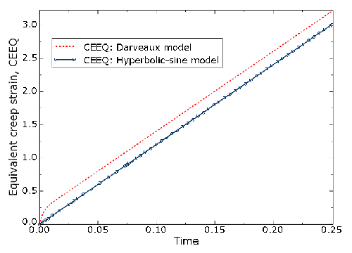
Hencky Hyperelastic Model
The Hencky model is an isotropic hyperelastic model that assumes a linear relation between the Kirchhoff stress tensor and the Hencky or logarithmic strain tensor. It is a generalization of the classical Hooke's law for isotropic infinitesimal elasticity. You define the model by providing two material parameters that can be measured at infinitesimal strains. The Hencky model can produce results that show good agreement with experimental data for a wide class of materials for moderately large deformations. You can also use the model as a finite strain alternative to the isotropic linear elastic model in situations where the isotropic linear elastic model is known to perform poorly (for example, for materials subjected to cyclic loads). In this case, the isotropic linear elastic material, which uses a rate formulation, might produce residual stresses when it returns to the initial (stress-free) configuration. The Hencky model does not show this undesirable behavior because it uses the total deformation to compute stresses.
Figure 1 shows a specimen subjected to simple shear cycling deformations with the mechanical response modeled using the Hencky and isotropic linear elastic models. Twenty cycles are performed with a different number of increments per cycle, and Figure 2 shows the Mises equivalent stresses. The results for the isotropic linear elastic material accumulate significant errors for a small number of increments per cycle, resulting in large residual stresses after a few cycles. They improve for larger numbers of increments per cycle and stabilize when the number increases to about 100. In contrast, the Hencky model shows no residual stresses even in the case where only two increments are used per cycle.

2024 FD01
Generalized Damage and Failure for Anisotropic Materials
Abaqus now provides a collection of stress/strain-based generalized damage initiation criteria as indicators of material failure. These general stress/strain-based damage initiation criteria are based on Tsai-Wu theory or maximum stress/strain theory. Abaqus does not support damage evolution laws for these damage criteria.
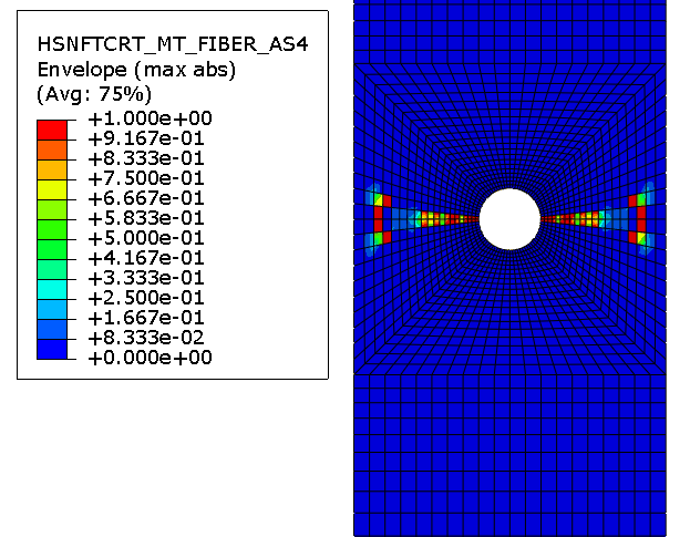
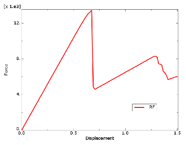
The figure below shows the failure index evaluated using the Tsai-Wu failure theory in an open hole tension test. The coupon plate is modeled with composite solid elements with [45/0/45/90]s layups.

The following figure shows the failure criteria evaluated using the Tsai-Wu stress and strain theory at the pseudo-grain level in an injection-molded plastic part. The maximum principal direction of the fiber orientation tensor is also shown below.

Damage and Failure for Fiber-Reinforced Composites Using Multiscale Modeling
Abaqus/Standard offers capabilities for predicting the onset of damage and for modeling progressive damage and failure at the constituent level in fiber-reinforced composites, which include unidirectional and woven fiber-reinforced composite materials. You can use the criteria with both 2D and 3D solid and shell stress/displacement elements. You can specify only linear responses in the constituents. You can also use the new damage initiation criteria in 3D elements; in earlier releases, these criteria were available for plane stress elements only.
The figures below show the results of an open hole tension test modeled with composite solid elements with [45/0/45/90]s layups. The top figure shows the fiber damage initiation criteria, and the bottom figure shows the reaction force result versus the displacement.
Field Expansion in Pore Fluid in a Porous Medium
In earlier releases, you could only define field expansion for the solid grains that make up the skeleton in a porous medium. Now, you can define field expansion in the different phases in a porous medium; that is, the solid grains and the pore fluid, independently. You can define only isotropic field expansion behavior for the pore fluid.
In addition, you can also output the strains due to both field expansion and thermal expansion in the pore fluid.
Band-Limited Damping in Abaqus/Standard
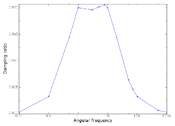
In many solid materials subjected to oscillatory loads, the energy dissipated in a cycle is controlled by internal friction and is insensitive to the frequency of the oscillation. This behavior cannot be captured by the stiffness proportional (beta) or mass proportional (alpha) damping options previously available in Abaqus/Standard, but can be modeled using the band-limited damping option. For this model, you specify the damping ratio, which can be defined as a function of temperature variables, field variables, or both. In addition, you provide the low and high frequency cutoff values to specify the frequency range, and Abaqus maintains approximately constant value of the damping ratio (and energy dissipated per cycle) within this range. In Abaqus/Standard, the effect of band-limited damping is considered only with the implicit dynamic procedure.
Figure 3 shows a bar subjected to harmonic excitations. The bar is fixed at the left end, and a displacement boundary condition is applied at the other end with different forced frequencies. The bar is modeled using a linearly elastic material in combination with band-limited damping. A constant damping ratio of 0.02 is specified, the low angular frequency is 1, and the high angular frequency is 10. Figure 4 shows the energy dissipated as a function of angular frequency, which remains approximately constant within the frequency range specified and decreases rapidly outside of the range. The damping ratio, obtained by scaling the energy dissipated in a cycle by the maximum value of the strain energy, is shown in Figure 5 and follows a similar pattern. As expected, Abaqus achieves a damping ratio approximately equal to 0.02 within the specified range of frequencies.