Material Damping

In direct-integration dynamic analysis you very often define energy dissipation mechanisms—dashpots, inelastic material behavior, etc.—as part of the basic model. In such cases there is usually no need to introduce additional damping: it is often unimportant compared to these other dissipative effects. However, some models do not have such dissipation sources (an example is a linear system with chattering contact, such as a pipeline in a seismic event). In such cases it is often desirable to introduce some general damping. Abaqus provides “Rayleigh” damping for this purpose. It provides a convenient abstraction to damp lower (mass-dependent) and higher (stiffness-dependent) frequency range behavior.

Rayleigh damping can also be used in direct-solution steady-state dynamic analyses and subspace-based steady-state dynamic analyses to get quantitatively accurate results, especially near natural frequencies.

To define material Rayleigh damping, you specify two Rayleigh damping factors: ${\alpha }_R$ for mass proportional damping and ${\beta }_R$ for stiffness proportional damping. In general, damping is a material property specified as part of the material definition. For the cases of rotary inertia, point mass elements, and substructures, where there is no reference to a material definition, the damping can be defined in conjunction with the property references. Any mass proportional damping also applies to nonstructural features (see Nonstructural Mass Definition).

For a given mode i the fraction of critical damping, ${\xi }_i$ , can be expressed in terms of the damping factors ${\alpha }_R$ and ${\beta }_R$ as:

where ${\omega }_i$ is the natural frequency at this mode. This equation implies that, generally speaking, the mass proportional Rayleigh damping, ${\alpha }_R$ , damps the lower frequencies and the stiffness proportional Rayleigh damping, ${\beta }_R$ , damps the higher frequencies.

For stiffness proportional damping, the fraction of critical damping is linearly proportional to the response frequency. Therefore, the desired damping ratio is achieved only at one target frequency. For practical purposes, it is useful to define the desired damping ratio uniformly over a reasonable frequency range. Band-limited damping provides this capability. It is available in Abaqus/Explicit and in Abaqus/Standard in implicit dynamic analysis.

Unlike stiffness proportional damping, which creates an additional damping stress proportional to the total strain rate, band-limited damping creates an additional damping stress, ${\mathit{\sigma }}_B$ . This additional damping stress is proportional to the rate of filtered constitutive stress at the integration point:

where

${\eta }_a$

is the actual damping ratio calculated based on the desired damping ratio and the frequency range,

$\sigma$

is the stress caused by the constitutive response at the integration point, and

$\dot{L}\mathrm{\{.\}}$

is the rate of linear transform $\mathrm{L\{.\}}$ , which is the low-pass filter operator.

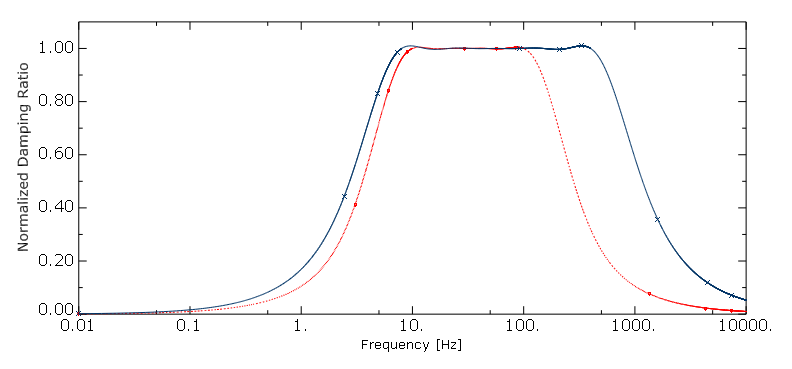
The frequency range is defined by the low-frequency cutoff, ${\mathit{f}}_l$ , and the high-frequency cutoff, ${\mathit{f}}_h$ . The actual damping ratio varies with frequency and achieves the desired damping ratio only within the frequency range. Outside the frequency range, the damping ratio is not exactly zero. The accuracy to achieve the desired damping ratio depends on the ratio of the high-frequency cutoff to the low-frequency cutoff, ${\mathit{f}}_h/{\mathit{f}}_l$ .

For example, if the desired damping ratio is ${\eta }_d$ , the normalized damping ratio is ${\mathit{\eta }}_a/{\mathit{\eta }}_d$ . Figure 1 shows the normalized damping ratio as a function of frequency for two cases: the red dotted line for the range ${\mathit{f}}_l\mathrm{=\; 10\; Hz}$ with ${\mathit{f}}_h/{\mathit{f}}_l\mathrm{=\; 10}$ , and the blue solid line for the range ${\mathit{f}}_l\mathrm{=\; 8\; Hz}$ with ${\mathit{f}}_h/{\mathit{f}}_l\mathrm{=\; 50}$ .

Figure 1. Normalized damping ratio.

It is well known that band-limited damping has a significant impact on the dynamic stiffness of the structure. The changes in the dynamic stiffness of the structure depend on the damping ratio and the frequency range. It increases the natural frequency of each mode, and the percentage change of the damped frequency could be large. For example, if ${\mathit{f}}_h/{\mathit{f}}_l\mathrm{=\; 100}$ , the maximum percentage change of the damped frequency to the natural frequency could reach approximately 1.65% (increased) with ${\eta }_d\mathrm{=0.02}$ . Compared to stiffness proportional damping, the percentage change of the damped frequency is only 0.02% (reduced). For the fixed ${\mathit{f}}_h/{\mathit{f}}_l$ , this percentage change is approximately linearly proportional to the damping ratio. Therefore, in practical applications, it is recommended that you use a low value for the damping ratio.

Similar to stiffness proportional damping, the band-limited damping stress is added to the stress caused by the constitutive response at the integration point when the dynamic equilibrium equations are formed, but it is not included in the stress output.

DAMPING, BAND LIMITED=${\eta }_d$, LOW FREQUENCY CUTOFF=$f_l$, 
HIGH FREQUENCY CUTOFF=$f_h$

DAMPING, BAND LIMITED=TABULAR, LOW FREQUENCY CUTOFF=$f_l$, 
HIGH FREQUENCY CUTOFF=$f_h$

Structural damping assumes that the damping forces are proportional to the forces caused by stressing of the structure and are opposed to the velocity. Therefore, this form of damping can be used only when the displacement and velocity are exactly 90° out of phase. Structural damping is best suited for frequency domain dynamic procedures (see Damping in Modal Superposition Procedures below). The damping forces are then

where $F_D^N$ are the damping forces, $i=\sqrt{-1}$ , s is the user-defined structural damping factor, and $I^N$ are the forces caused by stressing of the structure. The damping forces due to structural damping are intended to represent frictional effects (as distinct from viscous effects). Thus, structural damping is suggested for models involving materials that exhibit frictional behavior or where local frictional effects are present throughout the model, such as dry rubbing of joints in a multi-link structure.

Structural damping can be added to the model as mechanical dampers such as connector damping or as a complex stiffness on spring elements.

Structural damping can be used in steady-state dynamic procedures that allow for nondiagonal damping.

DAMPING, STRUCTURAL=$s$

Property module: material editor: MechanicalDamping: Structural: $s$

In Abaqus/Standard the operators used for implicit direct time integration introduce some artificial damping in addition to Rayleigh damping. Damping associated with the Hilber-Hughes-Taylor and hybrid operators is usually controlled by the Hilber-Hughes-Taylor parameter $\alpha$ , which is not the same as the ${\alpha }_R$ parameter controlling the mass proportional part of Rayleigh damping. The $\beta$ and $\gamma$ parameters of the Hilber-Hughes-Taylor and hybrid operators also affect numerical damping. The $\alpha$ , $\beta$ , and $\gamma$ parameters are not available for the backward Euler operator. See Implicit Dynamic Analysis Using Direct Integration for more information about this other form of damping.

Rayleigh damping is meant to reflect physical damping in the actual material. In Abaqus/Explicit a small amount of numerical damping is introduced by default in the form of bulk viscosity to control high frequency oscillations; see Explicit Dynamic Analysis for more information about this other form of damping.

As the fraction of critical damping for the highest mode ( ${\xi }_{\max }$ ) increases, the stable time increment for Abaqus/Explicit decreases according to the equation

where (by substituting ${\omega }_{\max }$ , the frequency of the highest mode, into the equation for ${\xi }_i$ given previously)

These equations indicate a tendency for stiffness proportional damping to have a greater effect on the stable time increment than mass proportional damping.

To illustrate the effect that damping has on the stable time increment, consider a cantilever in bending modeled with continuum elements. The lowest frequency is ${\omega }_{\min }=$ 1 rad/sec, while for the particular mesh chosen, the highest frequency is ${\omega }_{\max }=$ 1000 rad/sec. The lowest mode in this problem corresponds to the cantilever in bending, and the highest frequency is related to the dilation of a single element.

With no damping the stable time increment is

If we use stiffness proportional damping to create 1% of critical damping in the lowest mode, the damping factor is given by

This corresponds to a critical damping factor in the highest mode of

The stable time increment with damping is, thus, reduced by a factor of

and becomes

Thus, introducing 1% critical damping in the lowest mode reduces the stable time increment by a factor of twenty.

However, if we use mass proportional damping to damp out the lowest mode with 1% of critical damping, the damping factor is given by

which corresponds to a critical damping factor in the highest mode of

The stable time increment with damping is reduced by a factor of

which is almost negligible.

This example demonstrates that it is generally preferable to damp out low-frequency response with mass proportional damping rather than stiffness proportional damping. However, mass proportional damping can significantly affect rigid body motion, so large ${\alpha }_R$ is often undesirable. To avoid a dramatic drop in the stable time increment, the stiffness proportional damping factor, ${\beta }_R$ , should be less than or of the same order of magnitude as the initial stable time increment without damping. With ${\beta }_R=2/{\omega }_{\max }$ , the stable time increment is reduced by about 52%.

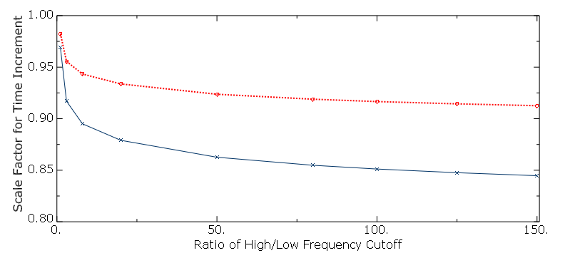
The above equation to calculate the stable time increment with critical damping is not suitable for band-limited damping. Because band-limited damping affects the dynamic stiffness of the structure, the stable time increment could have a dramatic drop if the damping ratio, ${\eta }_d$ , or the ratio of high-frequency cutoff to low-frequency cutoff, ${\mathit{f}}_h/{\mathit{f}}_l$ , is large. Figure 2 illustrates the scale factor for the stable time increment with band-limited damping. The red dotted line shows the scale factor as a function of ${\mathit{f}}_h/{\mathit{f}}_l$ with ${\eta }_d\mathrm{=0.02}$ , and the blue solid line shows the scale factor as a function of ${\mathit{f}}_h/{\mathit{f}}_l$ with ${\eta }_d\mathrm{=0.04}$ . For comparison, with stiffness proportional damping, the scale factor is 0.9801 when ${\xi }_{\max }\mathrm{=0.02}$ and is 0.9049 when ${\xi }_{\max }\mathrm{=0.04}$ , respectively.

Figure 2. Scale factor for the stable time increment in band-limited damping.

Damping can be specified as part of the step definition for modal superposition procedures. Damping in a Linear Dynamic Analysis describes the availability of damping types, which depends on the procedure type and the architecture used to perform the analysis, and provides details on the following types of damping:

• Viscous modal damping (Rayleigh damping and fraction of critical damping)

• Structural modal damping

• Composite modal damping

References

Huang, Y., R. Sturt, and M. Willford, “A Damping Model for Nonlinear Dynamic Analysis Providing Uniform Damping Over a Frequency Range,” Computer & Structures, vol. 212, pp. 101–109, 2019.