The mesh-independent fastener capability is a convenient method to define a localized
connection between two or more surfaces such as a spot weld or rivet connection.
In addition, the mesh-independent fastener capability:
uses spatial coordinates of fastener locations to define point-to-point connections
independent of underlying meshes;
combines either connector elements or BEAMMPCs with distributing coupling constraints to provide a
connection that can be located anywhere between two or more surfaces regardless of the
mesh refinement or location of nodes on each surface;
can be used to connect both deformable and rigid element-based surfaces;
can model either rigid, elastic, or inelastic connections with failure by using the
generality of connector behavior definitions; and
Many applications require modeling of point-to-point connections between parts. These
connections might be in the form of spot welds, rivets, screws, bolts, or other types of
fastening mechanisms. There might be hundreds or even thousands of these connections in a
large system model such as an automobile or airframe.
The fastener can be located anywhere between the parts that are to be connected regardless
of the mesh. In other words, the location of the fastener can be independent of the location
of the nodes on the surfaces to be connected. Instead, the attachment to each of the parts
being connected is distributed to several nodes in the surfaces to be connected in the
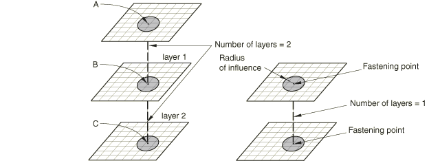
neighborhood of the fastening points. Figure 1 shows a typical one-layer and two-layer fastener configuration.
Figure 1. Typical one-layer and two-layer fastener configuration.
Each layer connects two fastening points using either a connector element or a BEAMMPC. Each fastening point is connected to the surface using
a distributing coupling constraint that couples the displacement and rotation of each
fastening point to the average displacement and rotation of the nearby nodes.
The mesh-independent fastener capability in Abaqus is designed to model these connections in a convenient manner. The fastener
automatically:
determines the locations of nodes and orientations of connector elements or BEAMMPCs between two or more surfaces;
generates distributing coupling constraints to attach the connector elements or BEAMMPCs to each surface in a mesh-independent manner; and
calculates weights for the distributing coupling constraints that complete the
mesh-independent connection.
For an example of the use of mesh-independent fasteners, see Buckling of a column with spot welds. Mesh-independent fasteners are referred to as point-based fasteners by
Abaqus/CAE. For more information, see About fasteners. It is also
possible to assemble fasteners in Abaqus/CAE using connector elements, coupling constraints, etc. For further details, see
About assembled fasteners.
Fastener Interactions
Fasteners are defined in groups called interactions, which are assigned names. Each
interaction defines one or more fasteners. The number of individual fasteners is equal to
the number of positioning points used to locate the fasteners. Fastening points on each
surface are found by considering the position of the positioning point as discussed in
subsequent sections.
Fasteners can be defined using connector elements or BEAMMPCs. BEAMMPCs allow modeling of perfectly rigid connectors between
components; while connector elements allow you to model much more complex behavior, such as
deformable connectors that include the effects of elasticity, damage, plasticity, and
friction.
For modeling perfectly rigid connections you need not define fasteners using connector
elements. Instead, Abaqus can internally generate BEAMMPCs connecting the fastening points of the fasteners. In
this approach you assign a reference node set containing a list of user-defined nodes to
the fastener interaction. The nodes in this reference node set will be used as positioning
points to locate the fasteners. If single-layer fasteners are to be modeled, Abaqus generates single BEAMMPCs with each node in the reference node set becoming
the first node of the BEAMMPC. The second node of each BEAMMPC will be generated internally by Abaqus. If multi-layer fasteners are to be defined, Abaqus generates linked sets of BEAMMPCs with each node in the reference node set becoming
the first node of the first BEAMMPC in each linked set. The subsequent nodes in each
linked set will be generated internally by Abaqus. For multi-layer fasteners each linked set contains as many BEAMMPCs as the number of layers in the fastener.
Input File Usage
Use the following options:
FASTENER, INTERACTION NAME=name,
REFERENCE NODE SET=node set labelNSET, NSET=node set label
Using connector elements as the basis for a point-to-point connection allows for very
complex behavior to be modeled with fasteners. Like other uses of connector elements, the
connection can be fully rigid or might allow for unconstrained relative motion in local
connector components. In addition, deformable behavior can be specified using a connector
behavior definition that can include the effects of elasticity, damping, plasticity,
damage, and friction. There are two methods to define fasteners that use connector
elements to model the behavior between fastening points. For both methods the fastener
interaction refers to an element set containing the connector elements. You must specify a
connector section definition that refers to this element set. You should be careful when
specifying the connector orientation (if needed) as discussed below in Defining the Fastener Orientation.
Defining the Connector Elements Directly
The most controlled approach to specifying fasteners using connector elements is to
define the connector elements explicitly and associate them with an element set. The
fastener interaction refers to the element set. Each fastener in the fastener
interaction corresponds to one or more connector elements depending on the number of
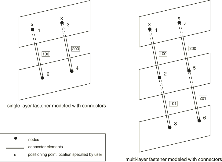
layers of the fastener (see Figure 2).
Figure 2. Single- and multi-layer fasteners modeled with connector elements.
A single connector element is associated with each layer, and the two nodes of the
connector element correspond to the fastening points of the two adjacent surfaces. When
specifying a multi-layer fastener, the connector elements for each layer should share
nodes with the connector elements of adjacent layers.
For a single-layer fastener the positioning point used to locate the fastener and its
fastening points is taken as the nodal coordinates of the first node of the connector
element. For a multi-layer fastener the positioning point is taken as the first node of
the first connector in a linked set of connectors with as many members as layers.
Examples of defining a single-layer and multi-layer fastener are included at the end of
this section.
Input File Usage
Use the following options:
FASTENER, INTERACTION NAME=name, ELSET=element set labelblank lineELEMENT, TYPE=CONN3D2, ELSET=element set labelCONNECTOR SECTION, ELSET=element set label
Abaqus/CAE Usage
For point-based fasteners in Abaqus/CAE, you cannot define the connector elements directly; the connector elements are
generated by Abaqus.
Connector Elements Generated by Abaqus
In this approach you do not need to explicitly define the connector elements that
connect the fastening points of the fastener. The fastener interaction refers to an
empty element set. You must specify a connector section definition that refers to this
element set. In addition, you assign a reference node set containing a list of
user-defined nodes to the fastener interaction. The nodes in this reference node set are
used as positioning points to locate the fasteners.
If single-layer fasteners are to be modeled, Abaqus generates single connector elements with each node in the reference node set becoming
the first node of a connector element. The second node of each connector element will be
generated internally by Abaqus. If multi-layer fasteners are to be defined, Abaqus generates linked sets of connector elements with each node in the reference node set
becoming the first node of the first connector element in each linked set. The
subsequent nodes in each linked set will be generated internally by Abaqus. For multi-layer fasteners each linked set contains as many connector elements as the
number of layers in the fastener. The connector elements are given internally generated
element numbers and assigned to the named user-specified element set. You can use this
element set to request output for these connector elements. However, this element set
should not be included in another element set definition.
Input File Usage
Use the following options:
FASTENER, INTERACTION NAME=name, ELSET=element set label,
REFERENCE NODE SET=node set labelblank lineNSET, NSET=node set labelCONNECTOR SECTION, ELSET=element set label
Example: Using Connector Elements to Define Single-Layer Fasteners Directly
To define a single-layer fastener directly using connector elements:
Define two connector elements with user element numbers 100 and 200 and
user-defined node numbers 1, 2 and 3, 4, respectively, and include them in an
element set. Nodes 1 and 3 act as the positioning points for the two fasteners (see
Figure 2).
Refer to the element set in the fastener interaction and connector section
definitions.
Assign section properties to the fasteners. Suppose in this example that relative
displacements between the fastening points are to be allowed. Therefore, the
fasteners must be assigned a section that has available components of motion; for
example, a CARTESIAN section can be used.
The relative displacement between the fastening points gives rise to elastic
deformations. Hence, the material between the fasteners is modeled as linear elastic
with a spring stiffness of 10000 using connector elasticity.
Example: Using Connector Elements to Define Multi-Layer Fasteners Directly
To define a multi-layer fastener directly using connector elements:
Define two linked sets of connector elements with each linked set containing
exactly two connectors. The first linked set comprises element numbers 100 and 101,
with node numbers 1, 2 and 2, 3, respectively. The second linked set comprises
element numbers 200 and 201, with node numbers 4, 5 and 5, 6, respectively. Include
the connector elements in an element set. Nodes 1 and 4 act as the positioning
points for the two fasteners (see Figure 2).
Refer to the element set in the fastener interaction and connector section
definitions
Assign section properties to the fasteners. Suppose in this example that rigid
beam-type behavior between the fastening points is to be modeled; in that case the
fasteners must be assigned a BEAM section.
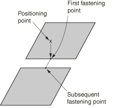
Specifying the Positioning Points, Projection Method, and Fastening Points
Each interaction defines one or more fasteners. The number of individual fasteners is equal
to the number of positioning points used to locate the fasteners. Positioning points are
nodes defined at the fastener locations and assigned as a reference node set to the
interaction.
In general, a positioning point should be located as close to the surfaces being connected
as possible. The reference node specifying the positioning point can be one of the nodes on
the connected surfaces or can be defined separately. Abaqus determines the actual points where the fastener layers attach to the surfaces that are
being connected by first projecting the positioning point onto the closest surface. Abaqus offers the following projection methods to find fastening points on the specified
surfaces to form fasteners:
Face-to-face
Face-to-edge
Edge-to-face
Edge-to-edge
Connector direction
The choice of method depends on how the surfaces are oriented relative to each other.
Fastening Surfaces That Are Nearly Parallel to Each Other
Most commonly the surfaces to be fastened together are nearly parallel to each other; in
which case the fastening points are located on element facets away from the periphery of
the surfaces. The face-to-face projection method is most appropriate for such situations.
It is also the default projection method.
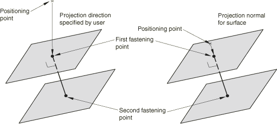
In the face-to-face projection method, Abaqus projects each positioning point onto the closest surface along a directed line segment
normal to the surface. Alternatively, you can specify the projection direction. Specifying
the direction might be useful when two-dimensional drawings are used to identify the
positioning point locations and those locations are known precisely in two dimensions but
not in a third. For this case the direction specified is typically the normal to the plane
of the drawing.
Once the fastening point on the closest surface has been identified, Abaqus determines the points on the other surface or surfaces to be connected by projecting
the first fastening point onto the other surfaces along the fastener normal direction,
which is typically normal to the closest surface. Figure 3 shows the two ways of locating the projection points. When surfaces to be fastened are
not exactly parallel, Abaqus sometimes sets attachment points to be at the closest facet edges or corner on the
surface, rather than along the fastener normal direction.
Figure 3. Directed and normal projection to locate the fastening points for the face-to-face
projection method.
The location of the positioning point (a node in the reference node set) might not
coincide with the locations of the fastening points found by Abaqus. Hence, the coordinates of the node at the positioning point might change from their
user-prescribed values when the node is shifted to a fastening point. If the node at the
positioning point is part of the connectivity of a user-defined element, this can cause
the element whose connectivity includes that node to undergo unacceptable initial
distortions. In such situations it is recommended that you define the node at the
positioning point separately. In general, you should not specify this node to be one of
the nodes of the connected surfaces.
Input File Usage
Use the following option to allow Abaqus to define the projection direction:
FASTENER, REFERENCE NODE SET=node set label, ATTACHMENT METHOD=FACETOFACE (default)
blank line
Use the following option to define the projection direction directly:
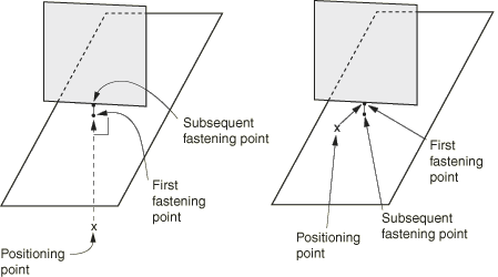
When you need to fasten surfaces that are perpendicular or nearly perpendicular to each
other; that is, forming a T-intersection, the face-to-edge or the edge-to-face projection
methods are appropriate choices. Figure 4 shows attachments for the face-to-edge and edge-to-face projection methods.
Figure 4. Face-to-edge and edge-to-face projection methods to locate fastening points for
surfaces that form T-intersections.
Creating the First Fastening Point on a Face
In the face-to-edge projection method Abaqus projects the positioning point onto the closest surface along a directed line segment
normal to the surface. The subsequent fastening points are found by searching for the
closest points on the remaining specified surfaces. The closest fastening point might
fall on the edge or a corner of a surface.
Input File Usage
FASTENER, REFERENCE NODE SET=node set label, ATTACHMENT METHOD=FACETOEDGEblank line
In the edge-to-face projection method, the first fastening point is found by searching
for the closest point on the specified surface or surfaces. The closest point might be
on the edge or corner of the surface. For subsequent fastening points Abaqus projects the previous fastening point along a directed line segment normal to the
surface.
Input File Usage
FASTENER, REFERENCE NODE SET=node set label, ATTACHMENT METHOD=EDGETOFACEblank line
When it is desired to form fasteners between surfaces that are butting against each
other, the edge-to-edge projection method is appropriate. In this method the first as well
as the subsequent fastening points are located by searching for the closest point on the
specified surface or surfaces. The fastening points in this method might be located on the
edge of a surface. Figure 5 shows attachments for the edge-to-edge projection method.
Figure 5. Edge-to-edge projection method to locate fastening points for abutting
surfaces.
Input File Usage
FASTENER, REFERENCE NODE SET=node set label, ATTACHMENT METHOD=EDGETOEDGEblank line
When fastening surfaces that are not parallel to one another, you can control the precise
location and direction of the fastener. To define the location and direction, prescribe a
connector element for each fastener with nodes at a specific location. Abaqus maintains the location and the direction of the connector element.
Input File Usage
FASTENER, ELSET=element set label, ATTACHMENT METHOD=CONNECTORDIRECTIONblank line
Abaqus/CAE Usage
Selecting a connector to control the location and direction of the fastener is not
supported in Abaqus/CAE.
Specifying the Surfaces to Be Fastened
Once the positioning points have been specified, the surfaces to be fastened can be
specified using two different approaches. In the first approach you directly specify the
surfaces that are to be connected with a fastener. In the second approach you specify a
search zone, and Abaqus automatically identifies the surfaces that are to be connected. However, in the second
approach Abaqus does not distinguish between coincident facets. Hence, if coincident facets are to be
fastened, you should specify distinct surfaces containing each of the coincident facets and
use the first approach. Only element-based surfaces defined on faces can be fastened
together (see Element-Based Surface Definition and Operating on Surfaces).
Forming Fasteners on User-Specified Surfaces
If you specify multiple surfaces as part of the interaction definition, the surfaces to
be fastened are restricted to these surfaces. In general, specifying multiple surfaces is
the preferred way of defining fasteners; this method leads to a more precise fastener
construct definition. The number of layers of each fastener is one less than the number of
surfaces specified. One fastening point is found on each surface.
Input File Usage
FASTENERfirst data linesurface1, surface2, surface3, etc.
Controlling Connectivity of Fasteners on User-Specified Surfaces
By default, the connectivity of the fastening points is determined by their relative
position along the fastener projection direction. For example, the default connectivity
for the two-layer example shown in Figure 1 connects fastening point A to point B (layer 1) and point B to point C (layer 2).
You can control the connectivity of the fastening points when the fasteners are formed on
user-specified surfaces. You can specify that the connectivity of the fastening points be
defined by the order in which you specified their associated surfaces.
Input File Usage
FASTENER, UNSORTEDfirst data linesurface1, surface2, surface3, etc.
If user-specified surfaces are not included on the data lines, the
UNSORTED parameter is ignored.
Forming Fasteners on Surfaces inside a User-Specified Search Zone
If you do not specify any surfaces as part of the interaction definition, Abaqus searches for fastening points on all element facets that fall within a sphere of
user-specified radius R with its center at the positioning point. If
you do not specify the search radius, Abaqus computes a default search radius based on five times the facet thickness (for shell
element facets) or the characteristic element length (for other element types) in the
vicinity of each positioning point.
To refine the search, you can specify a single surface definition that will limit the
facet search to element facets belonging to that surface. In this case you must define a
collective surface that includes at least each connected surface. A combined surface can
also be used (see Operating on Surfaces for a
discussion on combining surfaces).
To refine the search further, you can specify a positive integer value,
N, for the number of layers of each fastener. Abaqus searches for the fastening points closest to the positioning point. If BEAMMPCs are used to model the fastener, a warning message is
issued if the requisite number of fastening points is not found. However, if connector
elements are used to model the fastener and the requisite number of fastening points is
not found, Abaqus issues an error message. Thus, when specifying the number of layers, you should ensure
that the search radius has been specified such that fastening points can be found.
If multiple surfaces are listed as part of the fastener definition, the number of layers
for each fastener is ignored. If a user-specified search radius is used for the multiple
surface case, Abaqus searches for fastening points on all facets belonging to each of the listed surfaces
that fall within a sphere of user-specified radius R with its center
at the positioning point. Facets of the listed multiple surfaces that lie outside this
sphere are not included in the search. A maximum of 15 layers can be specified for a
particular fastener definition.
You should always examine the fastener definitions that Abaqus created to make sure that they are appropriate for your model.
Input File Usage
FASTENER, SEARCH RADIUS=R, NUMBER OF LAYERS=Nfirst data line
Abaqus/CAE Usage
Interaction module: SpecialFastenersCreate: Point-based: Criteria: Search radius: Specify: R, Maximum layers for projection: Specify: N
Defining the Radius of Influence
Each fastening point is associated with a group of nodes on the surface in the immediate
neighborhood of the fastening point called a region of influence. The motion of the
fastening point is then coupled in a weighted sense to the motion of the nodes in this
region by a distributed coupling constraint. Several weighting options are available and are
discussed in the next section.
To define the region of influence, Abaqus computes an internal radius of influence based on the geometric properties of the
fastener, the characteristic length of the connected facets, and the type of weighting
function used. The default radius of influence is always chosen to be the largest of the
internally computed radius of influence, the physical fastener radius, and the distance of
the projection point to the closest node. You can also specify the desired radius of
influence. However, Abaqus overrides a user-specified radius of influence that is smaller than the computed default
radius of influence. In any case each region of influence will contain a minimum of three
nodes.
The weighting methods available for the distributed coupling constraints created for a
fastener interaction are the same as those available for the surface-based coupling
constraints in Abaqus (see Coupling Constraints). Besides an area-based uniform weighting
scheme, various weighting methods are provided that monotonically decrease with radial
distance from the fastening point: linear, quadratic, and cubic polynomial weight
distributions. By default, Abaqus uses the uniform weighting method. You can modify the default weighting distribution.
The default radius of influence calculated by Abaqus is larger for higher-order weighting methods since the resulting weights for nodes away
from the fastening point contribute comparatively little to the motion of the fastening
point. Hence, to ensure that there is a sufficient “smearing” effect, it becomes necessary
to increase the number of nodes in the region of influence by increasing the size of the
default radius of influence. In comparison, for a uniform weighting scheme, surface nodes
away from the fastening point contribute significantly to the motion of the fastening point.
For this case the default radius of influence chosen can be comparatively small, since even
with a small number of nodes in the region of influence, the smearing effect is sufficiently
strong. If fewer than three cloud nodes are found, increasing the radius of influence might
help in forming the fastener by including more nodes in the cloud of coupling nodes.
Input File Usage
Use the following option to specify a uniform weight distribution:
Each fastener is formulated in a local coordinate system that rotates with the motion of
the fastener. By default, Abaqus defines the local system by projecting the global coordinate system onto the surfaces
that are being fastened according to the usual convention for surfaces in space (see Conventions). Local
directions specified in this manner are such that the local z-axis for
each fastener is normal to the surface that is closest to the reference node for the
fastener.
You can override the default local system by specifying a local coordinate system for the
fastener interaction. Generally, the user-defined orientation should be such that the local
z-axis of the orientation is approximately normal to the surfaces
that are being connected and the local x- and
y-axes are approximately tangent to the surfaces that are being
connected. By default, Abaqus adjusts the user-defined orientation such that the local z-axis for
each fastener is normal to the surface that is closest to the reference node for the
fastener. In cases where you wish to define the local directions precisely, you can specify
that Abaqus should not adjust them.
Fasteners support only rectangular, cylindrical, and spherical orientation definitions.
Additional rotations defined as part of the orientation definition are ignored.
In geometrically nonlinear analysis steps the local directions rotate with the motion of
the fastener reference node.
Local Coordinate System When Connector Elements Are Used
If a connector element is used to model a fastener, the local coordinate system defined
on the connector section, , operates on the local coordinate system for the fastener, , to determine the final local coordinate system of the connector
element, . In other words,
In the above equations and are assumed to be orthogonal rotation matrices with the local 1-, 2-,
and 3-directions being the first, second, and third rows, respectively. The local
coordinate system for a connector element modeling a fastener should be specified with
respect to the local coordinate system of the fastener. The
orientation displayed in the Visualization module of Abaqus/CAE (Abaqus/Viewer) is at all fastener locations unless you specify not
to write the orientations to the database; in this case, only is displayed. If connector or displacement field
output is requested, field output for additional nodal rotation at the connector nodes
is generated automatically to ensure that the appropriate connector orientation
directions are displayed as the analysis progresses. Otherwise, the orientation computed at the beginning of the analysis is
displayed at all times with the updated orientations used for computation
purposes.
For example, suppose you use a HINGE
connector and want the released rotational degree of freedom, which is in the connector's
local 1-direction, to be normal to the surfaces that are being fastened. If the default
local coordinate system is used for the fastener (local 3-direction normal to the
surface), the local 1-direction for the connector should be set to (0., 0., 1.); that is,
the local 3-direction of the fastener. When compounded with the local coordinate system
for the fastener, the local 1-direction for the connector will be normal to the surface.
See Mesh-independent spot welds for an example
of a compounded orientation.
Input File Usage
FASTENER, ORIENTATION=orientation name,
ADJUST ORIENTATION=NOblank line
Abaqus/CAE Usage
Interaction module: SpecialFastenersCreate: Point-based: Adjust: Fastener CSYS: Edit: select local coordinate system, toggle off Adjust CSYS to make local Z-axis normal to closest surface
Clarifications regarding the Computation of
A few clarifications regarding the default definition of are necessary for a precise understanding of the behavior when
connector elements are used to model fasteners. The positioning point is always
projected on the closest surface to be fastened. Therefore, the choice of coordinates of
the reference node relative to the stack of surfaces to be fastened determines which
surface is used to compute the local directions. Typically this choice does not matter
much in realistic applications because the surfaces to be fastened are more or less
parallel to each other in the fastener area.
The projection of the reference node on the closest surface generates a fastening point
for the connector element. The local z-axis for each fastener () is normal to the surface at this fastening point. The fastening point
generated on the closest surface is by default the first fastening point and, therefore,
the first connector node. The precise direction into which the local
z-axis is pointing is chosen such that the dot product with the
unit vector pointing from the first node of the connector to the second node of the
connector is positive. As explained above, you can control the connectivity of the
fastening points in the connectors by specifying unsorted surfaces. Therefore, you can
control the precise direction the local z-axis is pointing along
the surface normal by either selecting appropriate coordinates for the reference node
and/or by using unsorted surfaces.
The two tangential directions in are computed by default according to the usual convention for surfaces
in space (see Conventions). The global
X-axis is projected onto the closest surface at the location of
the fastening point to determine the local x-axis in . If the global X-axis is within 0.1 degrees of
being normal to the surface, the local x-axis in is the projection of the global Z-axis on the
closest surface. The local y-axis in is then at right angles to the local x-axis and
z-axis so that the three local axes form a right-handed set.
In the rare cases when the default definition of does not suit your application, you can always specify the orientation
directly. In this case the following occurs:
Abaqus first recomputes the local z-axis to align with the facet
normal, with the precise direction chosen such that its dot product with the unit
vector pointing from the first node of the connector to the second node of the
connector is positive.
Abaqus checks the local x- and y-axes you
specified to determine which of these two is closest to the plane of the current
facet.
If the local x-axis is closest, Abaqus recomputes the local y-axis as the normalized cross product
of the recomputed z-axis and the specified
x-axis. Then Abaqus computes the new local x-axis as the normalized cross
product of the recomputed y-axis and the recomputed
z-axis.
If the local y-axis is closest, Abaqus recomputes the local x-axis as the normalized cross product
of the specified y-axis and the recomputed
z-axis. Then Abaqus computes the new local y-axis as the normalized cross
product of the recomputed z-axis and the recomputed
x-axis.
Common Modeling Practices
In most applications the default choice for combined with a choice of global system for at both connector nodes would result in a that is most suitable. The connection type that you choose depends on
several modeling considerations, but very often the
BUSHING connection type offers the
best choice. To simplify the discussion, consider that only two surfaces are being
fastened, a very common situation as illustrated in the spot weld example in Connector Functions for Coupled Behavior. For this
common choice, has the local z-axis normal to the closest
surface and pointing from the first fastening point (first connector node) toward the
second fastening point (second connector node). This choice ensures that for a fastener
subjected to a tension load (fastened plates pulled apart) a positive force always
develops in the connector along the local z-axis
(CTF3) regardless of the choice of
coordinates for the positioning point and/or use of unsorted surfaces. Conversely, if a
compression load is applied (fastened plates pressed against each other), a negative
force develops in the connector.
In most cases, the behavior in the tangential plane defined by the local
x- and local y-axes is isotropic; therefore,
the precise orientation of these two axes is of less interest to you. The spot weld
example in Connector Functions for Coupled Behavior illustrates
such a typical case where the (isotropic) magnitude of two in-plane forces () and of the two moments () are used in the kinetic behavior of the connector element.
If you need to specify anisotropic behavior in the tangential plane, you need to
understand precisely how the directions in are defined. As explained above, the choice of coordinates for the
positioning point relative to the stack of surfaces to be fastened and/or use of
unsorted surfaces determines the precise direction of the default local axes. In most
cases you have two common modeling choices. In the first case you can specify the
coordinates of the positioning points to be exactly on or very close to the surface onto
which the first fastening points (connector nodes) are to be placed and use the default
sorted surfaces. In this case you do not need to specify the surfaces to be fastened
individually. However, in many practical situations imprecise geometry for the surfaces
to be fastened and/or inexact coordinates of the fastener reference nodes make the
consistent placement of the reference nodes in the vicinity of one particular surface
very hard to accomplish. The second modeling technique consists of using sorted
surfaces. The exact location of the reference node with respect to the surface stack to
be fastened is not that important because the first fastening point is always on the
first specified surface. In this case you do have to specify two or more individual
surfaces to be fastened. In the rare cases when neither of these modeling techniques
suits your application, you can specify the fastener orientation directly to match your
needs exactly.
Coupling Fasteners to Surfaces
Mesh-independent fasteners constrain the translation and rotation of each fastening point
to the average motion of the associated coupling cloud nodes of a fastened surface. The
cloud nodes follow the motion of the reference node in an average sense, with deformation
allowed among cloud nodes.
Translational and rotational constraints for the fastening points are formed similarly to
distributing coupling constraints, as described in more detail in Distributing Coupling Constraints. As for distributed
coupling constraints, the fastener couplings constraints are formed such that:
Cloud node translations always influence both translation and rotation of the
fastening point.
Cloud node rotations typically have a minor influence on the rotation of the fastening
point. This influence becomes more significant if cloud nodes are collinear or nearly
collinear (see Distributing Coupling Constraints).
The translational coupling constraint is such that translation of the weighted center
of the cloud corresponds to the average translation of the cloud nodes. By default, the
fastening point translation follows the weighted center translation plus the effect of
rotation of a rigid arm from the weighted center to the fastening point. This rigid-arm
rotation corresponds to the fastening point rotation. Cloud node rotational degrees of
freedom can participate in an additional offset term for the translational coupling
constraint, such that the fastening point remains close to a shell surface during
bending.
In many cases when the pair of fastened surfaces are close to each other, unrealistic
contact interactions might occur between the two surfaces unless an evolving offset
associated with bending is introduced in the translational coupling constraints. This
offset introduces the influence of cloud node rotational degrees of freedom into the
translational coupling constraints. For this coupling method to be active, all rotational
degrees of freedom at all coupling nodes must be active (as is the case when shells are
fastened together) and all degrees of freedom must be constrained (which is the default;
see Defining Fastener Properties below).
Use of this option is independent of whether or not cloud node rotations influence
rotational coupling constraints.
Controlling Whether Cloud Node rotations Influence Fastening Point Rotation
By default, Abaqus couples fastening point rotations to cloud node translations alone, unless all cloud
nodes are nearly collinear and have rotational degree of freedom. You can optionally
control whether or not the cloud node rotations influence the fastening point rotation.
However, these options are subject to the following conditions:
If the cloud nodes are collinear, Abaqus cannot couple the fastening point rotation about the axis of collinearity of the
cloud system to the cloud node translations alone. When this situation arises, Abaqus issues a warning message that identifies the axis about which the fastening point
rotation is not coupled to the cloud system. A consequence of the above is that a
component of moment about the axis of collinearity acting at the reference node will
not be transmitted to the cloud system.
If a cloud nodes are not nearly collinear and you force cloud node rotations to
influence fastening point rotation, the actual influence of cloud node rotations on
the fastening point rotation is typically insignificant. Some performance degradation
can occur due to appearance of additional terms in the coupling equations.
Input File Usage
Use the following option (default) to allow Abaqus to choose if the cloud nodes rotations should be included in the rotational
constraint:
A nondefault option for Abaqus/Standard to neglect cloud rotations in a rotational constraint for fastening points of
mesh-independent fasteners is not supported in Abaqus/CAE.
Defining Fastener Properties
Each fastener interaction definition must refer to a property, which defines the geometric
section properties of the fastener.
Interaction module: SpecialFastenersCreate: Point-based: Property: Physical radius: r
Releasing Degrees of Freedom on Fasteners Using Connector Elements
For fasteners modeled with connector elements, translational as well as rotational
degrees of freedom can be released by prescribing connector section types that have
unconstrained (available) degrees of freedom. For example, a
HINGE connector can be used to release
the rotational degree of freedom in the connector's local 1-direction.
Releasing Degrees of Freedom on Fasteners Using BEAMMPCS
For fasteners modeled with BEAMMPCs, the moment constraint between the rotation degrees
of freedom at the fastening points and the average rotation of the coupling nodes can be
released in one, two, or three directions. You can specify the moment constraint
directions in the default local coordinate system or a user-defined local coordinate
system. The three translational degrees of freedom at the fastening points are always
coupled to the average translation of the coupling nodes. You specify the degrees of
freedom of the fastening point to be coupled to the average motion of the coupling nodes
as part of the fastener property definition.
If no degrees of freedom are specified as part of the fastener property definition, all
six degrees of freedom are coupled. If you specify one or more degrees of freedom but not
all available translation degrees of freedom, Abaqus issues a warning message and adds all the available translation degrees of freedom to
the constraint. If a user-specified local orientation is specified for the fastener
interaction, the local degrees of freedom are with respect to the user-defined coordinate
system.
For example, if the default local coordinate system is used, the following property
definition would release the relative rotation constraint of the connected parts about
the surface normal:
The above property definition might be used to approximate a riveted
connection.
Abaqus/CAE Usage
Abaqus/CAE always constrains all translational degrees of freedom in a fastener. Use the
following input to remove constraints on the rotational degrees of freedom:
Interaction module: SpecialFastenersCreate: Point-based: Formulation: toggle off UR1, UR2, or UR3
Overconstraints in Fasteners Modeled with BEAMMPCS
There are several instances in which a model with fasteners modeled with BEAMMPCs might be overconstrained. Described below are two
potential overconstraints that Abaqus automatically attempts to detect and resolve during solver input file processing.
Fasteners and Rigid Bodies
Fasteners can be used to connect both deformable and rigid element-based surfaces.
However, if the fasteners are modeled with BEAMMPCs, potential overconstraints might arise if more than
one rigid surface is involved in a given fastener definition. Abaqus automatically attempts to remove these types of overconstraints by allowing at most one
rigid surface in any individual fastener definition. A warning message is generated if an
overconstraint of this type is detected.
For example, suppose surfaces A and C in Figure 1 are part of the same rigid body, and surface B is deformable. Abaqus automatically removes either surface A or surface C from the fastener definition and
only forms the fastener between the deformable surface and the remaining rigid surface. If
surface A and surface C belong to two separate rigid bodies, their respective rigid body
reference nodes will be joined by an internally generated BEAMMPC.
In another example, suppose all three surfaces in Figure 1 are rigid. In this case no fastener will be formed, and the unique rigid body reference
nodes for surfaces A, B, and C will be joined by beam
MPCs. Unresolvable overconstraints might arise if
inconsistent kinematic constraints (such as displacement boundary conditions) are placed
on rigid body reference nodes that have been joined by BEAMMPCs. In this case you must modify the model to resolve
the overconstraints. Possible courses of action include removing some of the rigid
surfaces from the fastener definitions or removing inconsistent kinematic conditions on
the rigid body reference nodes.
The above-described procedure to resolve overconstraints with fasteners and rigid bodies
will preserve the kinematics of the original model. In Abaqus/Standard you can bypass the overconstraint checks and prevent automatic model modifications in
the model preprocessor (see Overconstraint Checks).
Overlapping Fasteners
Potential overconstraints exist with rigid fasteners if all the coupling nodes of any
associated distributing coupling element are wholly contained within one or more other
fastener definitions. This can happen if the spacing between positioning points is small
compared to the typical element size in a mesh (which is often the case in automotive
models). To avoid overconstraints in this situation, Abaqus uses a penalty formulation for all fastener distributing coupling elements that satisfy
the above criteria. The penalty distributing coupling formulation relaxes, to a small
degree, the constraint between the motion of the distributing coupling element reference
node and its coupling nodes.
Output
If fasteners are modeled using connector elements, connector element output variables can
be used to request output for fasteners (see Connector Elements). No fastener
output is available if the fasteners are modeled using BEAMMPCs.