Analysis | ||
| ||
2025 GA
Step Cycling
The use of step cycling provides an efficient mechanism to loop over the sequence of steps with significant performance improvements. It also provides mechanisms to end a step sequence prematurely based on certain user-specified criteria. A step cycle sequence can be preceded or followed by steps and/or another cycle sequence.
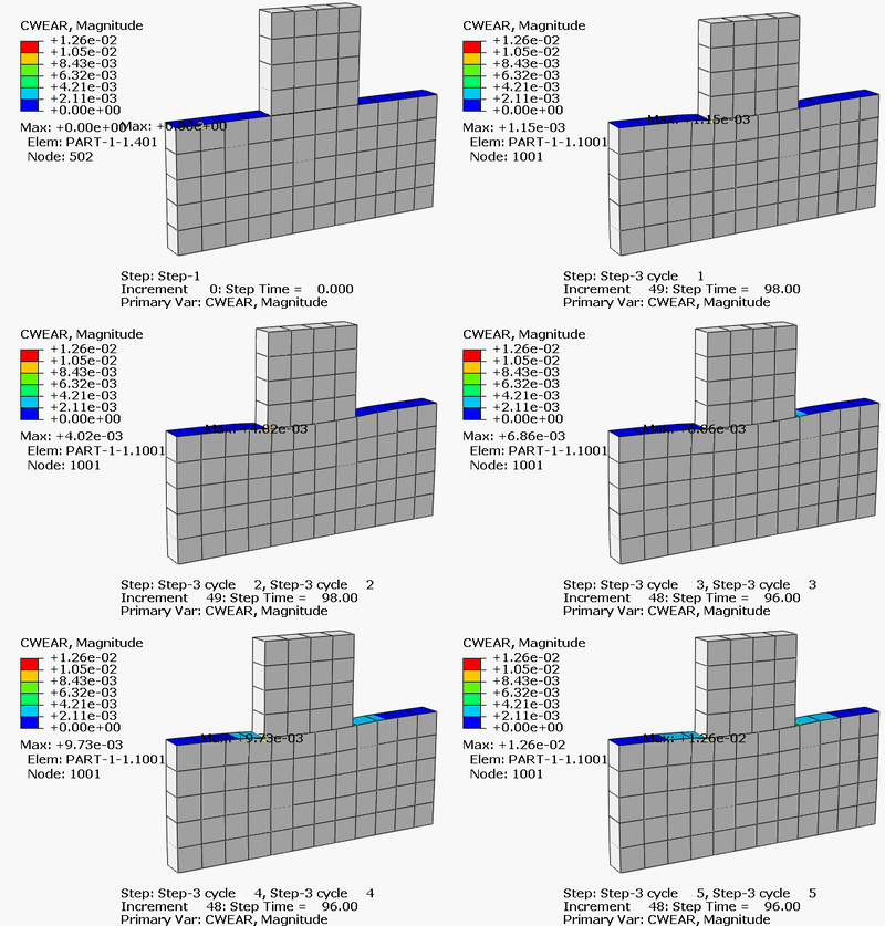
The figure above shows wear distance accumulation on the slider and the bottom block as the slider repeatedly moves back and forth. In this example, the sample wear cycle is modeled using two steps. In “Step-2” the slider moves to the right and returns to the center, while in “Step-3” the slider moves to the left and returns to the center. You can find additional details on this example in Step Cycling for Contact Wear Simulations.
2024 FD03
Alternative Convergence Checks
While the traditional convergence checks in Abaqus/Standard work well for structural simulations, they might be too restrictive for some multiphysics problems (such as battery electrochemistry simulations) that involve strong coupling among a number of different physical fields.
In earlier releases, the only way to modify the default convergence behavior in Abaqus/Standard was to specify nondefault tolerances on the maximum residuals and corrections during an increment. The new alternative convergence checks provide greater flexibility and can be used either globally (for all fields that are active in the analysis) or on an individual field basis. You can also modify the choice of the convergence checks at the step level.
| Important: The use of this set of features requires some experience and testing to ensure that the alternative convergence measures produce results with an acceptable level of accuracy. |
| Model | Number of DOFs | Iteration Count | Gain | |
|---|---|---|---|---|
| Convergence Check = Strict | Convergence Check = Relaxed | |||
| Model 1 | 792 | 1998 | 1662 | 1.20 |
| Model 2 | 2232 | 673 | 357 | 1.88 |
| Model 3 | 82692 | 156 | 128 | 1.22 |
| Model 4 | 2380141 | 1417 | 958 | 1.48 |
| Model 5 | 2764054 | 1998 | 1662 | 1.20 |
| Model 6 | 4457894 | 545 | 395 | 1.38 |
Adjoint Design Sensitivity Analysis
- Eigenfrequency adjoint design sensitivity analysis now supports the AMS eigensolver. In earlier releases, you could use only the Lanczos eigensolver for this analysis type. Now, you can run adjoint design sensitivity analyses for larger models and take advantage of parallel scaling in the AMS eigensolver.
- Direct steady-state dynamic adjoint design sensitivity analysis now supports topology and shape optimization. In earlier releases, you could use only sizing optimization for this analysis type.
- Direct steady-state dynamic adjoint design sensitivity analysis and eigenfrequency adjoint design sensitivity analysis now allow you to specify sizing and topology design variables for the same element.
State Space Solver for Transient Modal Dynamic Analysis
In earlier releases, the only solver available for transient modal dynamic analysis with nondiagonal modal damping was the conventional solver. The conventional solver uses a time integration scheme based on the assumption that the nondiagonal entries of the modal damping operator vary linearly within each time increment together with the loads. It calculates the approximate modal solution, and the solution accuracy depends on the time step size. In addition, the time integration algorithm is not unconditionally stable, particularly for models with a high level of damping. For common engineering simulations, the accuracy and stability of the conventional solver is usually acceptable. However, obtaining an accurate and stable solution using the conventional solver requires the use of very small time increments for specific cases. In addition, the conventional solver does not support coupled structural-acoustic analysis.
The new state space transient modal dynamic solver calculates the exact modal solution for systems with arbitrary modal damping for loads that vary piecewise linearly with time. This solver uses the complex eigenmodes of the unsymmetric modal state space operator to represent the real transient modal solution. The solution includes two phases: solving the unsymmetric eigenvalue problem for the state space operator at the “setup” phase and calculating the transient solution at the “apply” phase. The setup phase is the most computationally intensive part of the analysis. It can be costly for systems with many thousands of modes. However, the calculated solution with the state space solver is more accurate than for the conventional solver and the algorithm is unconditionally stable. In addition, the state space solver supports structural-acoustic transient modal analysis using the modal subspace built from the coupled structural-acoustic eigenmodes or from the uncoupled structural and acoustic eigenmodes.
Unit System Translation
To avoid mistakes, it is best to perform coupled multiphysics and multiscale simulation where both models use the same units. Abaqus has no units built into it and assumes self-consistent units. Some third-party solvers might represent their internal data in a unit system different from the one in which the user defined the model.
The SIMULIA Co-Simulation Engine typically tabs into the solver and consequently exchanges field data in the solver’s unit system. This forces the Abaqus model to be in the unit system used by the other solver’s internal format and can lead to unconventional model specification. For example, consider a sequential analysis of a circuit board modeled in CST Studio Suite with results imported into Abaqus. You might employ the CGS system (centimeter-gram-seconds) to define the electromagnetic model. However, CST Studio Suite converts everything to SI (International System) units to perform calculations. This forces the Abaqus model to be in SI units and to use meters as the length dimension for model definition (geometry, material data, load, etc.), which is an unconventional choice for this particular workflow.
Translation between unit systems is available only if the following are true:
- the unit system is defined in the Abaqus model and
- the other solver supports unit system translation through the co-simulation service.
DMP Direct Sparse Solver Enhancements
Performance improvements are expected in workflows dominated by the backward pass; for example,
- static substructure generation using the conventional (not AMS-based) algorithm,
- linear perturbation static or steady-state dynamic analysis with multiple load cases, and
- eigenvalue extraction using the Lanczos eigensolver.
The improvements also eliminate cases where the solver could stop responding in certain DMP configurations. While this enhancement improves performance of the backward pass when the factorized matrix resides entirely in system memory, it might degrade performance for cases where the factorized matrix must be partially stored on disk.
To demonstrate performance improvements, two benchmark models are run on Intel Xeon Gold 6348 (2.6 GHz Ice Lake processor with 56 physical cores), with 2 NUMA nodes, and 2 sockets.
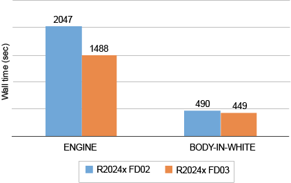
- Model 1: Static substructure generation for an engine model with 12M DOFs with 2028 retained DOFs run using a host configuration of 1 × 1 × 56 (1 node, 1 mpi rank, 56 threads). This model shows 1.4x speedup in 2024 FD03 compared to 2024 FD02.
- Model 2: Direct steady-state dynamic analysis for a body-in-white car model with 3.6M DOFs with 20 frequency points and 120 load cases run using a host configuration of 2 × 8 × 7 (2 nodes, 8 mpi ranks, 7 threads). This model shows 1.1x speedup in 2024 FD03 compared to 2024 FD02.
MPI-Based Parallel Execution of the Lanczos Eigensolver
You can now run frequency extraction analyses using the Lanczos eigensolver in a hybrid mode that utilizes both MPI and thread parallelism. By leveraging both MPI and thread parallelism within a single compute node, as well as across multiple compute nodes on the HPC cluster, the new Lanczos eigensolver significantly enhances the performance of Lanczos eigensolver workflows.
The figure below shows the performance improvement of Abaqus/Standard using the new Lanczos eigensolver in 2024 FD03 for four benchmark models. Each column represents an Abaqus/Standard run time in a different host configuration. Because of the new enhanced thread-based direct solver released in 2024 GA, the Lanczos eigensolver uses the new enhanced thread-based direct sparse solver in shared memory parallel (SMP) mode and the DMP direct sparse solver available in earlier releases in hybrid mode.
The figure illustrates the following:
- The Lanczos eigensolver in SMP mode in 2024 FD03 shows better performance than the previous version in 2024 FD02 for some of models due to the enhancements in the eigenmode transfer phase.
- The Lanczos eigensolver in hybrid mode in 2024 FD03 shows good parallel scaling using multiple MPI ranks on a single compute node. It also shows significantly improved performance compared to the eigensolver in 2024 FD02. For the full vehicle model with 2.5M DOFs, for example, Abaqus/Standard using a host configuration of 1 x 8 x 7 in 2024 FD03 shows 1.6 times speedup compared to 2024 FD02.
- For all four benchmark models, the Lanczos eigensolver in hybrid mode (1 x 8 x 7) runs faster than the Lanczos eigensolver in SMP mode. It also runs faster than the AMS eigensolver with full recovery for some models in 2024 FD03. Therefore, the new Lanczos eigensolver in hybrid mode surpasses the performance limitations of the eigensolvers in SMP mode.

The figure below illustrates the performance improvement of the new Lanczos eigensolver when utilizing multiple compute nodes on the HPC cluster as follows:
- The new Lanczos eigensolver shows good parallel scaling using multiple compute nodes.
- The new Lanczos eigensolver using multiple compute nodes (that is, using more CPU cores and memory) runs significantly faster than the Lanczos eigensolver and the AMS eigensolver in SMP mode for all four models.
- For the impeller model with 8.2M DOFs, for example, Abaqus/Standard using a host configuration of 3 x 8 x 7 in 2024 FD03 runs 1.6 times faster than the previous version in 2024 FD02. It is even faster than the AMS eigensolver in 2024 FD03. This demonstrates that the new Lanczos eigensolver in hybrid mode using multiple compute nodes surpasses the performance limitations of the eigensolvers in SMP mode.

Parallel Execution for SPH Progressive Element Conversion
Earlier releases of Abaqus/Explicit supported SPH progressive element conversion only in serial execution mode, limiting the usability of this feature for broad applications. This release supports parallel execution for SPH progressive element conversion, which enables you to take full advantage of the intrinsic strengths of both the Lagrangian finite element and SPH methods.
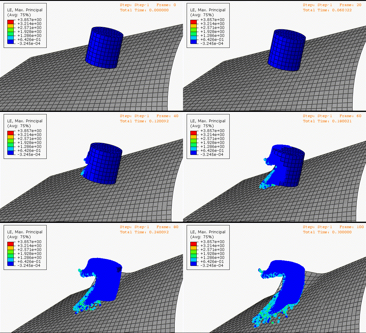
Figure 1 shows a parallel run example for a model of a bird striking an airplane engine blade. The bird structure consists of 480 C3D8R elements, with an EOS material definition that can be converted to around 100k SPH particles based on a strain conversion criterion. Once the strain for a certain C3D8R element meets the user-defined conversion criterion, the element is converted to SPH particles to sustain more severe deformation. The graphs in Figure 2 show the parallel execution speedup as function of the number of processors, illustrating reasonably good scaling.
The parallel speedup might vary for different models depending on the uniformity of the SPH particle distributions. It is recommended to use more uniform-sized parent elements (preferably C3D8R) for the SPH progressive element conversion to achieve better accuracy and parallel scalability.

Fatigue Crack Growth Analysis Using Field Import-Based Submodeling
2024 FD02
Element Design Responses for Transient Adjoint Design Sensitivity Analysis
In addition, you can use user subroutine UELEMDRESP to define a user-defined element design response, such as a failure criterion, in a transient optimization.
Specifying Design Responses in an Adjoint Design Sensitivity Analysis
The list of available operators for node and element design responses now includes the maximum absolute and the minimum absolute operators. These operators can be helpful in situations such as the following:
- In the context of node responses, the maximum absolute operator is useful when the nodal displacements for a node set that contains many nodes should be constrained to be less than a certain value. Without the maximum absolute operator, you must define one node response for each node in the node set, leading to many node responses (and corresponding adjoint sensitivities) in the output database. When you use the maximum absolute operator, you need to define only a single design response that uses this design objective or constraint.
- The minimum absolute operator is useful when the reaction force for a node set that contains many nodes must be larger than a certain value. Without the minimum absolute operator, you must define one node response for each node in the node set, leading to many node responses (and corresponding adjoint sensitivities) in the output database. When you use the minimum absolute operator, you need to define only a single design response that uses this design objective or constraint.
- You can now specify lower and upper bounds on the values of a design response outside of which Abaqus will not compute the adjoint sensitivities. By default, Abaqus writes the design response and the corresponding adjoint sensitivities to the output database for all design responses that do not have any prescribed bounds for the design response definition. In some situations, the sensitivities are necessary only if the value of a design response is within a certain range. In these cases, specifying the lower and upper bounds on the design response values provides a convenient way to limit the sensitivity calculations and the size of the output database.
Structure-to-Structure Co-Simulation Using Abaqus/Standard and Abaqus/Explicit
Co-simulation between Abaqus/Standard and Abaqus/Explicit exhibits strong physics coupling and requires special treatment at the co-simulation interface. The enhanced subcycling method (see Enhanced Subcycling Method for Interface Calculations), which improves solution robustness and is more computationally efficient, was introduced in an earlier release. The enhanced subcycling method is recommended over the original subcycling method (see Original Subcycling Method for Interface Calculations) and the lockstep method (see Lockstep Method for Interface Calculations).
The original subcycling method and the lockstep method used the *CO-SIMULATION, PROGRAM=ABAQUS option. Since these are no longer the recommended interface treatments, the PROGRAM=ABAQUS parameter is being deprecated. In addition, the *CO-SIMULATION CONTROLS option, which selects between the original subcycling and lockstep algorithms, is also being deprecated.
You can still select any of the above interface treatment methods by specifying the fields exchanged explicitly and by using the appropriate co-simulation service configuration file, as described in Structural-to-Structural Co-Simulation.
The image below shows a cantilever beam impacted by an object. The beam is split into
two domains: the orange portion is modeled in Abaqus/Standard, and the green portion is modeled in Abaqus/Explicit.
Full-Model Input for Abaqus Import
When you use the full-model input format, you give imported model data (such as nodes and elements, node sets and element sets, and sections and materials) in the input. This provides complete model information used in the import analysis.
By using the full-model input format, you can perform certain import workflows (such as importing a previously rigid element set as deformable) simply by omitting the rigid body definition of the element set in the import input. The following example illustrates this approach. The bolts are defined as rigid in the first analysis (left), and they are imported as deformable in the import analysis (right).

Undrained Pore Fluid Flow and Stress Analysis
A porous medium typically consists of a solid skeleton of numerous solid grains that are “loosely packed” and a permeating pore fluid that occupies a system of interconnected pores among these solid grains. You can ignore the effect of fluid flow in situations when the loading rate is significantly faster than the rate at which pore fluid can drain from the porous medium. This corresponds to the undrained conditions.
The undrained pore fluid flow and stress analysis functionality in Abaqus/Explicit is intended for the simulation of fully saturated porous media under undrained conditions. The functionality enables modeling the increase in stiffness of the soil in applications such as trenching, gouging, and pile driving. In these applications, you can ignore fluid diffusion terms when the rate of loading is fast compared to the characteristic time of the diffusion process.
2024 FD01
Iterative Solver Performance Improvements
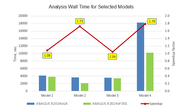
The new domain decomposition algorithm takes into account the connectivity of the finite element model, the element formulation details, and the material properties. It creates a better clustering of elements with similar properties and separates out clusters with dissimilar properties. This makes it easier for the iterative solver to find a smooth solution in individual aggregates, which results in improved convergence rates overall. The algorithm optimizes the load balance between domains for large models in parallel runs by accounting for the actual computational costs of different elements. The solution time reduction due to the improved domain decomposition varies from model to model. The improvement can be moderate for some finite element models, but it can be significant for large-scale models with complicated geometry using higher-order element formulations.
The figure below illustrates the improved performance of the iterative solver for four selected finite element models:
- Model 1: airplane fuselage structure; shell-dominated finite element model with 48.3 million degrees of freedom.
- Model 2: powertrain model with 23.6 million degrees of freedom meshed with linear continuum elements.
- Model 3: powertrain model with 11.2 million degrees of freedom meshed with quadratic continuum elements.
- Model 4: battery model with 46.0 million degrees of freedom, meshed with linear continuum, shell, and connector elements.
Generating Reduced Bases for Use with Nonlinear Flexible Multi-Body Systems
A reduced basis is a set of basis vectors that can represent solutions from preceding analysis cases when they are superimposed with according scaling factors. You can now generate reduced bases for use in downstream nonlinear flexible MBS simulations with Simpack as follows:
- Define a nonlinear static analysis case that ramps up a large deformation of a flexible component in a shape that is characteristic for its behavior in downstream system simulations. For example, apply a distributed load that acts on the surface of a wind turbine rotor blade in the flap-wise direction, or define a spring support for a twist beam axle and apply a twisting load at the wheel attachment points.
- Output the operator data at various deformation levels.
- Add natural frequency extraction steps at various deformation levels.
- Add the reduced basis generation step.
The reduced basis generation step computes the reduced basis from the solution data and computes the auxiliary operator data from all the preceding analysis steps. The reduced basis and projected operator data are written to a SIM (.sim) file. Optionally, you can write a Simpack Flexible Body Interface (.fbi) file with a complete Simpack nonlinear flexible body definition that you can assign directly to a nonlinear flexible body in Simpack.
Random Response Analysis Performance Improvements
The enhancement substantially improves performance of the following phases of the random response analysis:
- Reading the eigenfrequency extraction stresses.
- Computing the element results. New scalable algorithms perform the element output computations.
In addition, you can now use the frequency split technique to run a random response analysis on models that do not require calculations of the root-mean-square variables.
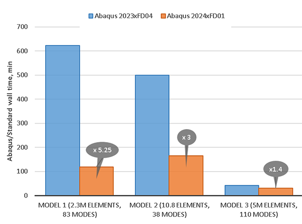
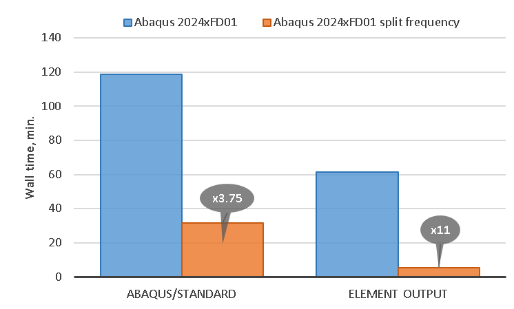
Figure 4 illustrates the wall time reductions for three industrial models, and Figure 5 illustrates the reduction in the wall time for the element results computation phase for the same three models.
The models and results are as follows:
- Model 1 is comprised of 2.3 million elements containing approximately 9 million
degrees of freedom. The random response analysis was performed using 83 eigenmodes
and 840 frequency points. Stress field output was requested in all increments.
The Abaqus/Standard wall time was reduced approximately 5.25 times, while the element results computation phase was sped up approximately 9 times.
- Model 2 is comprised of 10.8 million elements containing approximately 53 million
degrees of freedom. The random response analysis was performed using 38 eigenmodes
and 20 frequency points. Stress and strain field output was requested in all
increments.
The Abaqus/Standard wall time was reduced approximately 3 times, while the element results computation phase was sped up approximately 10 times.
- Model 3 is comprised of 5 million elements containing approximately 25 million
degrees of freedom. The random response analysis was performed using 110 eigenmodes
and 38 frequency points. Stress and Mises stress field output was requested in 0.6
million elements at all frequency points.
The Abaqus/Standard wall time was reduced approximately 1.4 times, while the element results computation phase was sped up approximately 3.6 times.
Figure 6 shows the result of applying the frequency split technique to Model 1. The 840 frequency points used for the random response analysis were split into 16 batches. The total Abaqus/Standard wall time (that includes the wall time of a frequency extraction step and the largest wall time of the random response analyses) was reduced approximately 3.75 times, while the element results computation phase was reduced approximately 11 times.

AMS Eigensolver Performance Improvement
The performance of the following phases related to full eigenmodes recovery is significantly improved for the AMS eigensolver workflow including the AMS-based substructure generation procedure:
- AMS recovery phase
- Constraint transformation and recovery phases
- Substructure recovery matrix output phase
The figure below illustrates the performance improvement of Abaqus/Standard in Abaqus 2024 FD01 for four industrial models. In this figure, the blue columns represent the Abaqus 2023 GA run time, and the orange columns represent the Abaqus 2024 FD01 run time.
The models and results are as follows:
- Model 1 is a heavy-duty engine model with 15.2 million degrees of freedom,
extracting 10 eigenmodes below 100Hz and 5,704 substructure modes for 5,704 retained
degrees of freedom.
Abaqus 2024 FD01 shows a 36% performance improvement over Abaqus 2023 GA.
- Model 2 is a powertrain model with 26.3 million degrees of freedom, extracting 6
eigenmodes below 500Hz and 1,512 substructure modes.
Abaqus 2024 FD01 shows a 22% performance improvement over Abaqus 2023 GA.
- Model 3 is a full vehicle model with 54.6 million degrees of freedom, extracting
1,630 eigenmodes below 150Hz and 1,984 substructure modes.
Abaqus 2024 FD01 shows a 39% performance improvement over Abaqus 2023 GA.
- Model 4 is a vehicle trim body model with 31 million degrees of freedom,
extracting 2,598 eigenmodes below 200Hz.
Abaqus 2024 FD01 shows a 38% performance improvement over Abaqus 2023 GA.

AMS Eigensolver GPU Acceleration
The figure below shows the GPU acceleration performance of Abaqus/Standard for a 7.6 million degree of freedom stator model that requires 2.3 × 10¹⁵ floating-point operations to factorize four system operators (including viscous and structural damping matrices). The blue columns represent the Abaqus 2023 GA run time, and the green columns represent the Abaqus 2024 FD01 run time. The performance data was obtained on a machine equipped with Intel Xeon Gold 6336Y (Ice Lake, 2.4GHz, 48 cores) processors, 512 GB physical memory, and 2x NVIDIA A100 (40 GB memory) cards.

Abaqus/Standard using the AMS eigensolver shows good parallel scaling up to 48 CPUs. However, using 16 CPUs and 2 GPUs results in the best performance of the GPU acceleration for this model.
Scalable Spectral Solver for Mode-Based Steady-State Dynamics Analysis
You can use the new spectral solver for the special cases of mode-based steady-state dynamic simulations. For all cases, you can apply any kind of structural damping in the model. The special cases are defined by the complementary viscous damping properties.
| Case 1 | No viscous damping | No material, global, or modal viscous damping |
| No dashpot elements, connector damping, or substructures with viscous damping | ||
| No matrix input data for the viscous damping | ||
| No other possible sources of the viscous damping | ||
| Case 2 | Low rank viscous damping operator | Viscous damping is defined locally in the model, for example, using dashpot elements, connector damping, or substructures with viscous damping |
| Structural-acoustic coupled steady-state dynamic analysis using uncoupled eigenmodes when the number of acoustic modes is significantly smaller than the number of the structural modes | ||
| Modal viscous damping defined for selected modes |
You can use the spectral solver for mechanical, acoustic, and structural-acoustic analyses. Using the spectral solver can be beneficial for models with the mentioned special damping properties when many eigenmodes and many points in the frequency domain are used for the frequency response calculation.
The spectral solver algorithm consists of two analysis phases: the Setup Solver Phase and the Apply Solver Phase. The computational cost of the Setup Solver Phase depends on the number of the eigenmodes, and it can be significant when that number is high. The computational cost of the Apply Solver Phase is proportional to the number of the frequency points specified for the frequency response calculation, and the solution calculation at a frequency point is relatively cheap. Therefore, the spectral solver can be less effective for the analyses with a small number of frequency points (when the setup phase dominates), but it can be very effective for the same model when more frequency points are used.
The figure below shows the performance benefits from using the new spectral modal solver over the conventional (default) solver that solves the system of equations with a dense complex matrix and multiple right hand sides at every frequency point. It compares the wall-time ratios for a steady-state dynamic analysis using the conventional and the new spectral solvers for the following models:
| Model | DOF | Load Cases | Eigenmodes | Frequency Points | Damping Properties | Cores | ||
|---|---|---|---|---|---|---|---|---|
| 1 | Body-in-white | 3.6 million | 120 | 12200 | 1000 | Material structural damping; no viscous damping | 40 | |
| 2 | Full vehicle | 9.7 million | 165 | 8800 uncoupled eigenmodes including 1000 acoustic modes | 1000 | Material structural damping; viscous damping — 6 dashpots | 40 | |
| 2000 | ||||||||
| 3 | Body-in-white | 35.6 million | 21 | 33800 | 1000 | Material structural damping; viscous damping —70 dashpots | 40 | |
| 56 | ||||||||
| 4 | Body-in-trim | 2.6 million | 110 | 11000+ | Uncoupled structural and acoustic eigenmodes | 1000 | Material structural damping; viscous damping — 6 dashpots | |
| Fully coupled structural-acoustic eigenmodes | ||||||||
| 5 | Fuselage model | 48.3 million | 120 | 21300 | 1000 | Material structural damping; no viscous damping | 40 | |
| 56 | ||||||||

Beam-Based Submodeling from Global Beam Elements to Shell Elements
Beam-to-shell submodeling is often a good strategy to study details in one or more local regions if a global model uses beam elements. Figure 7 shows a local shell-element model superimposed with beam elements from a global model. The shell thickness is rendered in Figure 7. This simple example is provided to demonstrate the concept; typically, the global model would be larger and more complex than shown here.

Beam-to-shell submodeling is similar to the beam-to-solid submodeling capability introduced in Abaqus 2023 FD03; in both cases distributing couplings are used to impose conditions from the global model at submodel cuts. For comparison, Figure 8 shows a local solid-element model superimposed with beam elements from a global model. Representations of distributing couplings at submodel cuts are shown in Figure 7 and Figure 8. Reference nodes of these distributing couplings are used to impose conditions from the global model on the submodel. Figure 9 shows the global model with beam cross-sections rendered.
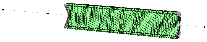

Figure 10 provides a comparison of displacement contour plots for the beam-element global model and each of the submodels.

Figure 11 shows Mises stress contour plots for each of the submodels.

2024 GA
Python 3
Formation of Tie Constraints in Import Analysis
The new protocol also guarantees formation of the same tie constraints for the surfaces in the import analysis as in the original analysis. It is used regardless of whether you specify the original or the updated configuration as the reference configuration for import.
Adjoint Sensitivity Analysis for Sizing Optimization in Direct Steady-State Dynamic Analysis
Abaqus/Standard now supports sizing optimization for select design variables (beam radii and shell thicknesses) in direct steady-state dynamic analyses for select design responses (nodal displacements/velocities/accelerations/rotations). You can define the range of frequencies over which you wish to compute the sensitivities for a particular design response.
You can use this new capability only for jobs run on a single domain and for node sets with nodes corresponding only to independent degrees of freedom.