Mechanical contact interactions can cause surface wear (erosion) due to
various microscale mechanisms, such as in abrasion and fretting.
Such mechanisms
are modeled in a continuum by phenomenological approaches that characterize the evolution of
wear.
Wear modeling:
uses variants of Archard's wear model to predict the rate of surface erosion based on
wear properties assigned to surfaces and contact conditions;
accounts for local surface wear distances in contact penetration calculations but not in
underlying element calculations;
is supported for both general contact and contact pairs in Abaqus/Standard and for general contact in Abaqus/Explicit;
can be used together with ALE adaptive meshing in Abaqus/Explicit (see About ALE Adaptive Meshing and );
can be used together with step cycling in Abaqus/Standard
supports wear accumulation in general steps with exceptions for steady-state transport
and locations with material transport boundary conditions; and
Wear is a microscale phenomenon triggered by mechanical contact resulting in
cumulative loss of surface material. One or both surfaces of a contact interface
might experience wear. Wear of analytical rigid surfaces is not supported. Wear
coefficients are specified as surface properties. Archard’s wear model is used such
that the wear distance rate at a given location is proportional to the wear
coefficient, contact stress, and slip rate. Wear often
occurs over large numbers of physical cycles with wear rates gradually evolving.
Efficient simulation of wear often calls for each cycle simulated to represent
multiple physical cycles.
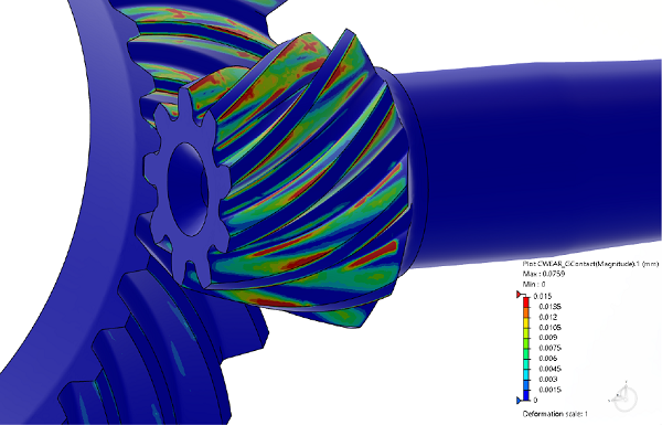
Small to moderate wear distances can be modeled accurately without
ALE by treating accumulated wear distances as nodal
offsets for contact penetration calculations, without affecting the underlying
element calculations (as shown, for example, in Figure 1).
Figure 1. Simplified helical bevel gear analysis.
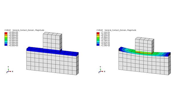
Wear modeling can be used together with Arbitrary Lagrangian-Eulerian (ALE) Adaptive
Meshing in Abaqus/Explicit such that surface geometry reflects accumulated wear and underlying elements are
smoothed, as explained in Enabling Adaptive Meshing (ALE) for Wear in Abaqus/Explicit. Figure 2
demonstrates use of ALE in the context of wear modeling; in this model most wear
occurs on the smaller block, with the maximum wear distance being approximately half
of the original element depth. ALE mesh smoothing is effective in providing a
realistic representation of the evolving part geometry and maintaining good mesh
quality.
Figure 2. Effect of ALE with wear in a slider example.
Wear Rate Models
Abaqus provides four versions of Archard’s wear rate model shown in Table 1.
First, consider the expression for surface wear rate with a dimensionless wear
coefficient that depends explicitly on the friction coefficient:
Frictional stress is if the (plastic) slip rate is nonzero, such that the wear rate can
be written as
corresponds to a frictional energy density dissipation rate, ; therefore, in this case the surface wear rate is proportional to
the frictional energy density dissipation rate:
is associated with contact, whereas the ratio is associated with surfaces. Incremental surface wear distances
might differ across an interface due to differences in among surfaces; however, incremental wear for each surface of an
interface is driven by local values of with this version of Archard's model. Of course, is zero for surface locations where is zero.
Other forms of Archard’s model shown in Table 1
are provided for cases in which the damage mechanism is more closely related to
contact pressure than frictional stress or for cases in which experimental data for
characterizing wear coefficients is gathered without consideration of material
hardness. Surface wear coefficients might depend on wear distance, contact pressure,
temperature, and field variables. For example, dependence of a wear coefficient on
the local wear distance can be useful for modeling wear of a part with a protective
surface coating. The wear coefficient can be specified to increase after erosion of
the protective coating.
In Abaqus/Standard, wear accumulation on surfaces in active contact is restricted to contact
formulations where portions of surfaces come into contact. Consequently,
supplementary formulations (the edge-to-surface, edge-to-edge, and vertex-to-surface
formulations) in general contact do not accumulate contact wear. Linear perturbation
steps also do not accumulate wear.
Table 1. Alternate versions of Archard’s wear equation.
Dimensionless wear coefficient
Lumped wear coefficient with dimensions
No friction coefficient dependence
Explicit friction coefficient dependence
Specifying Wear Properties
You can define named surface wear properties to assign them to individual surfaces.
You can also specify various attributes to each wear property to choose from one of
the alternative versions of Archard’s wear equation.
Input File Usage
Use the following options to create a named surface property and to define the
wear properties:
SURFACE PROPERTY, NAME=surface_wear_property_nameWEAR SURFACE PROPERTIES, UNITLESS WEAR COEF=YES or NO(default),
FRIC COEF DEPENDENT=YES or NO(default), REFERENCE STRESS=real_value, DEPENDENCIES=integer_value
For contact pairs, assign named surface wear properties to the individual surfaces of
the contact pair. Both element-based and node-based surfaces support wear property
assignments.
Input File Usage
Use the following option to assign named surface wear properties to a
surface:
Here, surface surf_A is assigned surface wear
property WEAR1, while surface
surf_B is assigned surface wear property
WEAR2. If surfaces
surf_A and surf_B,
overlap, the last wear assignment WEAR2 applies
in the overlap region (similar to how overlaps are handled for other property
types on the SURFACE PROPERTY ASSIGNMENT
option).
Abaqus/CAE Usage
Interaction module: Edit Interaction: General contact: Surface properties Tab: choose Global wear surface property assignment or Wear surface property assignment
Accounting for Wear with Nodal Offsets in Contact Calculations
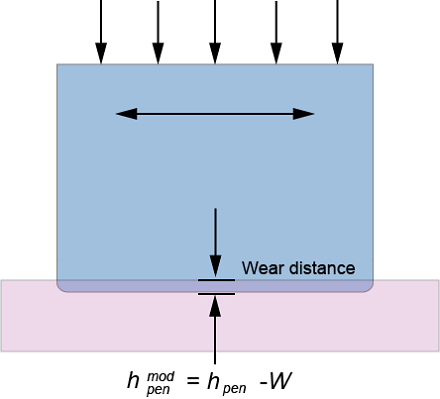
Figure 3
shows two parts in contact. The penetration distance accounting for wear, , corresponds to the penetration distance of the surfaces
neglecting wear, , minus the combined wear distances of the individual contact
surfaces, . In the absence of ALE, these wear distance offsets represent
total accumulated wear. For cases in which ALE mesh smoothing occurs periodically,
these wear distance offsets represent wear since the most recent ALE mesh
adjustments account for wear. Modifications to contact penetrations affect contact
stress calculations and, thereby, influence underlying element stresses. Abaqus uses accumulated wear distances from the previous increment to modify
penetrations in the current increment.
Figure 3. Contact penetration distance accounting for surface wear.
Strategies to Model Wear Accumulating Over Large Numbers of Cycles
Many wear contexts involve accumulation of wear over a large number of cycles. For
example, bearings might undergo millions of rotational cycles as wear gradually
accumulates during their service life. Efficient simulation of wear over a large
number of physical cycles calls for each simulation cycle to approximate effects of
multiple physical cycles. The ability to repeat an Abaqus step or a sequence of Abaqus steps until a stopping condition is satisfied (such as reaching a target maximum
wear distance) also facilitates the simulation of wear over a large number of
cycles.
Simple Strategy for Lumping Multiple Physical Wear Cycles into One Simulated
Cycle
A simplistic approach to lumping “N” physical wear cycles into one simulated
cycle is to include a scale factor of “N” in the specified wear coefficients.
This approach is used in Abaqus/Explicit. Several sliding cycles are simulated in one Abaqus/Explicit step in this case, but each of these simulated cycles might represent N=1000
(or another number of) physical cycles. Contact stress distributions gradually
evolve across wear cycles, which influences local wear rates. The number of
physical wear cycles represented per simulated cycle should be small enough to
integrate local wear rates across cycles accurately.
Using a Step Sequence for Modeling Wear
In Abaqus/Standard you can repeat a step or step sequence until a stopping condition is met,
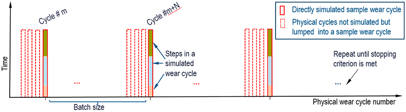
which is often convenient for modeling wear. Figure 4
represents repeating a step sequence, with each step sequence representing a
batch of physical wear cycles, until a stopping condition is met. Each vertical
bar in Figure 4
represents a physical wear cycle numbered along the horizontal axis. The
vertical axis denotes the simulation time for each wear cycle. The heights of
the vertical bars are the same because the loading history is repetitive. The
solid vertical bars represent wear cycles that are simulated directly and
approximate effects of a batch of physical cycles scaling the wear coefficient
based on the number of physical cycles represented. The groups of dotted
vertical bars next to the solid bars show batches of physical wear cycles that
are not simulated directly. Depending on the batch size, only a few sample
simulation cycles might be needed to make accurate wear predictions associated
with a large number of physical cycles.
Figure 4. Physical and sample simulated wear cycles for wear accumulation.
When modeling wear with this approach, you would typically specify:
the number of physical cycles to be represented by the first simulation
cycle;
a target value of the maximum incremental wear distance per simulated cycle;
and
a stopping condition, such as the maximum total wear.
The number of physical cycles represented by the second and subsequent simulated
cycles is automatically adjusted based on the incremental wear that occurred
during the previous sample simulation cycle.
When you use this approach, you should prescribe boundary conditions in rate form
(such as velocities) in case the beginning and ending configurations of a
simulation cycle do not match.
In the example below, a sample wear cycle is modeled with two general steps with
names WearStep-1 and WearStep-2. These two
steps will cycle as follows:
The step cycling sequence can be repeated up to 10 times.
The initial batch size is 10,000 cycles.
The upper bound on the batch size is 25,000 physical cycles.
In addition, step cycling controls are used to specify wear-based stopping
conditions for the step cycling loop and target values for the maximum
incremental wear distance per simulated cycle for two different node sets.
Input File Usage
Use the following to activate step cycling to repeat sample wear cycles
and to control early termination and automatic calculation of batch sizes
using step cycling controls:
Enabling Adaptive Meshing (ALE) for Wear in Abaqus/Explicit
The Arbitrary Lagrangian-Eulerian (ALE) adaptive meshing method offers a way to
incorporate wear effects into underlying element calculations, especially when wear
distances become significant relative to element dimensions.
For contact surfaces with wear properties, the motion of the nodes is imposed by the
nodal wear distance like a spatial mesh constraint and not by the adaptive meshing
algorithm. Between adaptive meshing increments (by default, every 10 increments),
wear is accounted for with nodal vectors that are considered in penetration
calculations; when the ALE increment is triggered, the accumulated wear distance
translates into actual mesh node motion.
Output
When you request contact wear output variable
CWEAR, the accumulated wear
vectors at the contact surface nodes are available either as field or history output
in Abaqus/Standard and as field output in Abaqus/Explicit.
Input File Usage
Use the following options to request field output: