The adaptive meshing technique in Abaqus combines the features of pure Lagrangian analysis and pure Eulerian analysis.
This type of adaptive meshing is often referred to as Arbitrary Lagrangian-Eulerian
(ALE) analysis. The Abaqus documentation often refers to “ALE adaptive meshing” simply
as “adaptive meshing.”
ALE adaptive meshing is a tool that makes it possible to
maintain a high-quality mesh throughout an analysis, even when large deformation or loss of
material occurs, by allowing the mesh to move independently of the material.
ALE adaptive meshing does not alter the topology (elements
and connectivity) of the mesh, which implies some limitations on the ability of this method to
maintain a high-quality mesh upon extreme deformation. Refer to About Adaptivity Techniques for a comparison between
ALE adaptive meshing and other Abaqus adaptivity methods.
ALE adaptive meshing is distinct from the pure Eulerian
analysis capability in Abaqus/Explicit. The pure Eulerian capability supports multiple materials and voids within a single
element, which allows effective handling of analyses involving extreme deformation (such as
fluid flow). In contrast, ALE elements are always 100% full
of a single material; while this formulation limits the deformation of material in the model
to the deformation of the elements, it allows more precise definitions of material boundaries
and more complex contact interactions. For more information on pure Eulerian analysis, see
Eulerian Analysis.
Although the adaptive meshing techniques and the user interface are similar in Abaqus/Explicit and Abaqus/Standard, the use-cases and the level of functionality are different. Adaptive meshing in Abaqus/Explicit is intended to model large-deformation problems. It does not attempt to minimize
discretization errors in small-deformation analyses. Adaptive meshing in Abaqus/Standard is intended for use in acoustic domains and for modeling the effects of ablation, or wear,
of material. A comparison between the adaptive remeshing functionality in Abaqus/Explicit and Abaqus/Standard is provided in this section.
Features of ALE Adaptive Meshing
ALE adaptive meshing:
can often maintain a high-quality mesh under severe material deformation by allowing
the mesh to move independently of the underlying material; and
maintains a topologically similar mesh throughout the analysis (that is, elements are
not created or destroyed).
In Abaqus/ExplicitALE adaptive meshing:
can be used to analyze Lagrangian problems (in which no material leaves the mesh) and
Eulerian problems (in which material flows through the mesh);
can be used as a continuous adaptive meshing tool for transient analysis problems
undergoing large deformations (such as dynamic impact, penetration, and forging
problems);
can be used as a solution technique to model steady-state processes (such as extrusion
or rolling);
can be used as a tool to analyze the transient phase in a steady-state process;
can be used in wear analysis to affect underlying element calculations; and
can be used in explicit dynamics (including adiabatic thermal analysis) and fully
coupled thermal-stress procedures.
In Abaqus/StandardALE adaptive meshing:
can be used to solve Lagrangian problems (in which no material leaves the mesh) and to
model effects of ablation, or wear (in which material is eroded at the boundary);
can be used to update the acoustic mesh when structural preloading causes significant
geometric changes in the acoustic domain; and
can be used in geometrically nonlinear static, steady-state transport, coupled pore
fluid flow and stress, and coupled temperature-displacement procedures.
Activating ALE Adaptive Meshing
Adaptive meshing can be applied to an entire model or to individual parts of a model. A
Lagrangian adaptive mesh domain will be created, so that the domain as a whole will follow
the material originally inside it, which is the proper physical interpretation for most
structural analyses. Additional options are provided for controlling the mesh. In Abaqus/Explicit analyses you can define Eulerian boundaries to allow material to flow into or out of the
domain modeled.
The subsequent sections of ALE Adaptive Meshing describe the various options that can be used
with adaptive meshing. Although these options give you the ability to exercise detailed
control over adaptive meshing, they are not necessary for many Lagrangian problems.
To take full advantage of all the adaptive mesh features in Abaqus, it is important to understand the concepts of adaptive mesh domains, boundary
regions, boundary edges, geometric features, and mesh constraints. These concepts are
explained in Defining ALE Adaptive Mesh Domains in Abaqus/Explicit and Defining ALE Adaptive Mesh Domains in Abaqus/Standard. Instructions for applying boundary conditions, loads, and
surfaces to adaptive mesh boundaries are also provided in those sections.
ALE Adaptive Meshing and Remapping in Abaqus/Explicit and ALE Adaptive Meshing and Remapping in Abaqus/Standard
outline the methods used to move the mesh and to remap solution variables to the new
mesh. These sections also present options for controlling these algorithms. Although the
default methods have been chosen to work well for a wide variety of problems, you may
wish to override the defaults to balance the robustness and efficiency of adaptive
meshing or to extend the use of adaptive meshing to relatively difficult or unusual
applications.
Step module: OtherALE Adaptive Mesh DomainEdit: toggle on Use the ALE adaptive mesh domain below, and click Edit to select the region
Uses for ALE Adaptive Meshing
Adaptive meshing is of great value in a variety of problems. Abaqus/Explicit and Abaqus/Standard each employ adaptive meshing in ways that provide the greatest value within the
particular solver.
Uses in Abaqus/Explicit
In problems where large deformation is anticipated the improved mesh quality resulting
from adaptive meshing can prevent the analysis from terminating as a result of severe mesh
distortion. In these situations you can use adaptive meshing to obtain faster, more
accurate, and more robust solutions than with pure Lagrangian analyses.
Adaptive meshing is particularly effective for simulations of metal forming processes
such as forging, extrusion, and rolling because these types of problems usually involve
large amounts of nonrecoverable deformation. Because the final shape of the product can be
drastically different from the original shape, a mesh that is optimal for the original
product geometry can become unsuitable in later stages of the process when large material
deformation leads to severe element distortion and entanglement. Element aspect ratios can
also degrade in zones with high strain concentrations. Both of these factors can lead to a
loss of accuracy, a reduction in the size of the stable time increment, or even
termination of the problem.
Uses in Abaqus/Standard
You can use adaptive meshing to enable acoustic domain meshes to follow the large
deformations of the bounding structure. In other applications you can use adaptive meshing
and adaptive mesh constraints to model arbitrarily large amounts of ablation of material
away from the domain.
Adaptive meshing of acoustic regions greatly extends the utility of acoustic analysis
procedures. Abaqus can be used to model the response of a coupled structural-acoustic system subjected to
structural preloads. By default, the structural-acoustic calculations are based on the
original configuration of the acoustic domain. This approximation is adequate as long as
the boundary between the fluid and structure does not experience large deformation during
application of the preload. However, when the geometry of the acoustic domain changes
significantly as a result of structural loading, the original acoustic configuration must
be updated. An example is the interior cavity of a tire subjected to inflation, rim
mounting, and footprint pressure loads.
The acoustic elements in Abaqus do not have mechanical behavior and, therefore, cannot model the deformation of the
fluid when the structure undergoes large deformation. Abaqus/Standard solves the problem of computing the current configuration of the acoustic domain by
periodically creating a new acoustic mesh that uses the same topology as the original mesh
but with the nodal locations adjusted so that the deformation of the structural-acoustic
boundary does not lead to severe distortion of the acoustic elements.
The geometric changes associated with the new acoustic mesh are then taken into account
in a subsequent coupled structural-acoustic analysis. However, it is assumed that the
material properties of the fluid, such as the density, do not change as a result of mesh
smoothing.
Adaptive meshing can also model effects of ablation, or wear, by enabling you to define
boundary mesh motions independent of the underlying material motion. An example is the
wearing of a tire during its life, an effect that can significantly affect the performance
of the structure.
Comparison of ALE Adaptive Meshing in Abaqus/Explicit and Abaqus/Standard
Adaptive meshing in Abaqus/Explicit is generally more robust and provides more features for controlling the mesh than does
adaptive meshing in Abaqus/Standard.
ALE Adaptive Meshing in Abaqus/Explicit
Adaptive meshing in Abaqus/Explicit is designed to handle a large variety of problem classes, and employs a variety of
smoothing methods, with controls that you can use to tailor the adaptivity to specific
problems. The Abaqus/Explicit implementation allows you to do the following:
to create entirely Eulerian models;
to improve the quality of the mesh initially, before deformation begins; and
to define tracer particles, which enable tracking and output of material-based
results quantities.
ALE Adaptive Meshing in Abaqus/Standard
Adaptive meshing in Abaqus/Standard uses a single smoothing algorithm that works well for structural acoustic analyses and
the modeling of ablation processes. The Abaqus/Standard implementation of adaptive meshing has the following limitations:
Initial mesh sweeps cannot be used to improve the quality of the initial mesh
definition.
The method is not intended to be used in general classes of large-deformation
problems, such as bulk forming.
Diagnostics capabilities are currently limited.
Illustrative Examples
To illustrate the value of adaptive meshing, simple examples of transient and steady-state
forming applications follow. For simplicity, two-dimensional cases are shown. In each case
Abaqus/Explicit is used in the simulation.
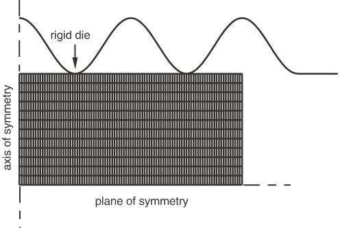
Axisymmetric Forging
In this example a well-lubricated rigid die of sinusoidal shape moves down to deform a
blank of rectangular cross-section (see Figure 1).
Figure 1. A blank and a sinusoidal die.
The indentation depth is 80% of the original blank thickness. Material extrudes upward
and outward (radially) as the blank is indented. The die is modeled with an analytical
rigid surface, and the blank is modeled with axisymmetric continuum elements in a regular
mesh configuration. The blank is assumed to have elastic-plastic material properties.
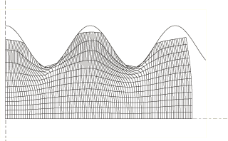
A pure Lagrangian analysis of this problem does not run to completion because of
excessive distortion in several elements, as shown in Figure 2. The contact surface cannot be treated correctly because of the gross distortion of the
elements at the troughs of the sinusoidal rigid surface.
Figure 2. Eventually, the purely Lagrangian analysis will terminate because of excessive
element distortion.
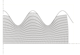
Adaptive meshing allows the problem to run to completion. A Lagrangian adaptive mesh
domain is created for the entire blank. Abaqus/Explicit automatically chooses suitable defaults for adaptive meshing; hence, the adaptive mesh
approach requires only two additional input lines:
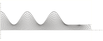
Figure 3 and Figure 4 show the deformed mesh at various stages of the forming analysis. Because the mesh
refinement is maintained on the areas of the secondary surface that contact the die
troughs as the material flows radially, contact conditions are resolved correctly
throughout the analysis.
Figure 3. Deformed configuration at an intermediate stage of the analysis. Figure 4. Deformed configuration upon completion of the analysis.
Steady-State Rolling Example
This example shows how adaptive meshing can be used in a steady-state simulation to allow
the flow of material through Eulerian boundaries on the problem domain. A steel plate is
passed through a symmetric roll stand to reduce its height by 50%. This simulation is run
until it reaches steady-state conditions.
Figure 5 and Figure 6 show the initial and final (steady-state) configurations in a purely Lagrangian model
of this problem.
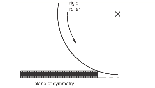
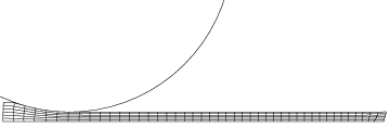
Figure 5. The initial configuration of the roller and the undeformed blank in the pure
Lagrangian model. Figure 6. The final steady-state configuration in the pure Lagrangian model.
Figure 7 shows this problem modeled using an Eulerian adaptive mesh domain, where material flows
through the mesh.
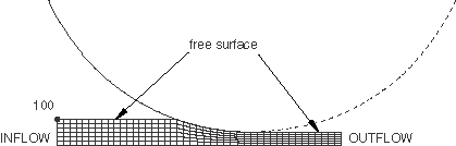
Figure 7. The initial Eulerian adaptive mesh domain.
Only the region near the roller is modeled. The exact location of the free surface does
not need to be known to set up the problem: it is created in a likely location, and the
final steady-state position is found as part of the solution. Although not shown, a
focused mesh can be used to capture steep strain gradients directly beneath the roller.
The Eulerian domain reaches the same steady-state solution as obtained with the Lagrangian
approach.
The Eulerian adaptive mesh domain is created by defining an inflow and an outflow
boundary on the adaptive mesh domain. Adaptive mesh constraints are applied normal to
these boundaries so that material will flow through the mesh (see Defining ALE Adaptive Mesh Domains in Abaqus/Explicit). Frictional contact between the roller and the blank
pulls material through the adaptive mesh domain.
The problem is set up by making the following modifications to the input file for the
pure Lagrangian analysis:
HEADING
...
ELSET, ELSET=BILLET
...
ELSET, ELSET=INFLOW
...
ELSET, ELSET=OUTFLOW
...
NSET, NSET=INFLOW
...
NSET, NSET=OUTFLOW
...
SURFACE, NAME=INFLOW, REGION TYPE=EULERIAN
INFLOW, S1
SURFACE, NAME=OUTFLOW, REGION TYPE=EULERIAN
OUTFLOW, S2
***************************
STEPDYNAMIC, EXPLICITData line to specify the time period of the step
...
ADAPTIVE MESH, ELSET=BILLET, CONTROLS=ADAPT
ADAPTIVE MESH CONTROLS, NAME=ADAPT
ADAPTIVE MESH CONSTRAINT, TYPE=DISPLACEMENT
INFLOW, 1, 1, 0.0
100, 2, 2, 0.0
OUTFLOW, 1, 1, 0.0
...
END STEP