Transient Modal Dynamic Analysis

Modal Dynamic Analysis

Transient modal dynamic analysis gives the response of the model as a function of time based on a given time-dependent loading. The structure's response is based on a subset of the modes of the system, which must first be extracted using an eigenfrequency extraction procedure (Natural Frequency Extraction). The modes will include eigenmodes and, if activated in the eigenfrequency extraction step, residual modes. The number of modes extracted must be sufficient to model the dynamic response of the system adequately, which is a matter of judgment on your part.

The modal amplitudes are integrated through time, and the response is synthesized from these modal responses. For linear systems the modal dynamic procedure is much less expensive computationally than the direct integration of the entire system of equations performed in the dynamic procedure (Implicit Dynamic Analysis Using Direct Integration).

As long as the system is linear and is represented correctly by the modes being used (which are generally only a small subset of the total modes of the finite element model), the method is also very accurate because the integration operator used is exact whenever the forcing functions vary piecewise linearly with time. You should ensure that the forcing function definition and the choice of time increment are consistent for this purpose. For example, if the forcing is a seismic record in which acceleration values are given every millisecond and it is assumed that the acceleration varies linearly between these values, the time increment used in the modal dynamic procedure should be a millisecond.

The user-specified maximum number of increments is ignored in a modal dynamic step. The number of increments is based on both the time increment and the total time chosen for the step.

While the response in this procedure is for linear vibrations, the prior response can be nonlinear and stress stiffening (initial stress) effects will be included in the response if nonlinear geometric effects were included in the step definition for the base state of the eigenfrequency extraction procedure, as explained in Natural Frequency Extraction.

Selecting the Modes and Specifying Damping

You can select the modes to be used in modal superposition and specify damping values for all selected modes.

Selecting the Modes

You can select modes by specifying the mode numbers individually, by requesting that Abaqus/Standard generate the mode numbers automatically, or by requesting the modes that belong to specified frequency ranges. If you do not select the modes, all modes extracted in the prior eigenfrequency extraction step, including residual modes if they were activated, are used in the modal superposition.

Input File Usage

Use one of the following options to select the modes by specifying mode numbers:

SELECT EIGENMODES, DEFINITION=MODE NUMBERS
SELECT EIGENMODES, GENERATE, DEFINITION=MODE NUMBERS

Use the following option to select the modes by specifying a frequency range:

SELECT EIGENMODES, DEFINITION=FREQUENCY RANGE

Abaqus/CAE Usage

You cannot select the modes in Abaqus/CAE; all modes extracted are used in the modal superposition.

Specifying Modal Damping

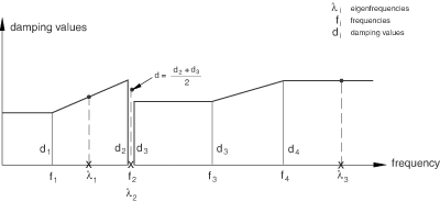
Damping is almost always specified for a mode-based procedure; see Material Damping. You can define a damping coefficient for all or some of the modes used in the response calculation. The damping coefficient can be given for a specified mode number or for a specified frequency range. When damping is defined by specifying a frequency range, the damping coefficient for a mode is interpolated linearly between the specified frequencies. The frequency range can be discontinuous; the average damping value will be applied for an eigenfrequency at a discontinuity. The damping coefficients are assumed to be constant outside the range of specified frequencies.

Input File Usage

Use the following option to define damping by specifying mode numbers:

MODAL DAMPING, DEFINITION=MODE NUMBERS

Use the following option to define damping by specifying a frequency range:

MODAL DAMPING, DEFINITION=FREQUENCY RANGE

Abaqus/CAE Usage

Use the following input to define damping:

Step module: Create Step: Linear perturbation: Modal dynamics: 
Damping

Example of Specifying Damping

Figure 1 illustrates how the damping coefficients at different eigenfrequencies are determined for the following input:

MODAL DAMPING, DEFINITION=FREQUENCY RANGE
 $f_{1}, d_{1}$ 
 $f_{2}, d_{2}$ 
 $f_{2}, d_{3}$ 
 $f_{3}, d_{3}$ 
 $f_{4}, d_{4}$

Rules for Selecting Modes and Specifying Damping Coefficients

The following rules apply for selecting modes and specifying modal damping coefficients:

No modal damping is included by default.
Mode selection and modal damping must be specified in the same way, using either mode numbers or a frequency range.
If you do not select any modes, all modes extracted in the prior frequency analysis, including residual modes if they were activated, will be used in the superposition.
If you do not specify damping coefficients for modes that you have selected, zero damping values will be used for these modes.
Damping is applied only to the modes that are selected.
Damping coefficients for selected modes that are beyond the specified frequency range are constant and equal to the damping coefficient specified for the first or the last frequency (depending which one is closer). This is consistent with the way Abaqus interprets amplitude definitions.

Specifying Global Damping

For convenience you can specify constant global damping factors for all selected eigenmodes for mass and stiffness proportional viscous factors, as well as stiffness proportional structural damping. Structural damping is a commonly used damping model that represents damping as complex stiffness. This representation causes no difficulty for frequency domain analysis such as steady-state dynamics for which the solution is already complex. However, the solution must remain real-valued in the time domain. To allow users to apply their structural damping model in the time domain, a method has been developed to convert structural damping to an equivalent viscous damping. This technique was designed so that the viscous damping applied in the frequency domain is identical to the structural damping if the projected damping matrix is diagonal. For further details, see Modal dynamic analysis.

Input File Usage

GLOBAL DAMPING, ALPHA=factor, BETA=factor, STRUCTURAL=factor

Abaqus/CAE Usage

Defining damping by global factors is not supported in Abaqus/CAE.

Material Damping

Structural and viscous material damping (see Material Damping) is taken into account in a transient modal analysis. The projection of damping operators onto the mode shapes is performed only one time during the frequency extraction step. If the damping operators depend on frequency, they will be evaluated at the frequency specified for property evaluation during the frequency extraction procedure.

Controlling Damping

You can deactivate the structural or viscous damping in a transient modal procedure if desired.

You can also control damping of the low frequency eigenmodes in transient modal analyses. This control is useful for free structures and models with secondary base motions, and it controls all sources of damping including the modal damping. To include low frequency eigenmodes, set the low frequency cutoff value to a small negative value. To exclude them, either provide a low frequency cutoff value or allow Abaqus to calculate it; it will be six orders of magnitude smaller than the eigenfrequency of the first deformable eigenmode.

Input File Usage

Use the following option to deactivate structural and viscous damping in a specific transient modal dynamic step:

DAMPING CONTROLS, STRUCTURAL=NONE, VISCOUS=NONE

Use the following option to control damping of the low frequency eigenmodes in a specific transient modal dynamic step:

DAMPING CONTROLS, LOW FREQUENCY CUTOFF

Abaqus/CAE Usage

Damping controls are not supported in Abaqus/CAE.

Transient Modal Dynamic Solver

The basic concept of the modal superposition method is that the equations of motion of the finite element model are projected onto the modal subspace. Solving the projected modal equations of motion yields the modal solution: generalized displacements, velocities, and accelerations as functions of time. The response of the structure is expressed in terms of the mode shape vectors and the modal solution.

If the finite element model is not damped or if only modal and/or global damping are specified:

the projected modal damping operator is diagonal, and
the modal equations of motion are uncoupled.

Abaqus/Standard uses the diagonal transient modal dynamic solver in that case. The modal response is integrated through time: Abaqus/Standard calculates the exact solution of the uncoupled differential equations of motion assuming that all the loads vary piecewise linearly within each time increment. This calculation is very fast and stable.

If damping is introduced at the finite element level, the modal damping operator might not be diagonal. For example, when damping is specified as the material property or when dashpots or connectors with damping are used in the model, the damping operator is nondiagonal. When the modal damping operator is nondiagonal, Abaqus/Standard calculates the modal solution using either the state space or the conventional solver.

Abaqus/Standard selects the transient modal dynamic solver automatically and uses the diagonal solver whenever possible. For analyses with nondiagonal modal damping, Abaqus/Standard uses the state space solver by default. You can overwrite this default by selecting the conventional solver. In general, this is not recommended, unless the number of modes is very high and the state space solver setup phase is too costly. In addition, using the conventional solver for models with high levels of damping is not recommended.

State Space Transient Modal Dynamic Solver

The state space transient modal dynamic solver calculates exact modal solution for systems with arbitrary damping for loads that vary piecewise linearly with time. This solver uses the complex eigenmodes of the unsymmetric modal state space operator to represent the real transient modal solution. Obtaining the solution includes two phases:

solving the unsymmetric eigenvalue problem for the state space operator at the “setup” phase and
calculating the transient solution at the “apply” phase.

The setup phase is the most computationally intensive part of the analysis. It can be costly for systems with many thousands of modes. The calculated solution is more accurate than that obtained using the conventional solver, and the algorithm is stable.

The state space solver supports structural-acoustic transient modal analysis using the modal subspace built from the coupled structural-acoustic eigenmodes or the uncoupled structural and acoustic eigenmodes.

Input File Usage

Use the following option to select the state space transient modal dynamic solver (default):

MODAL DYNAMIC, SOLVER=STATE SPACE

Abaqus/CAE Usage

The state space transient modal dynamic solver is the default solver in Abaqus/CAE.

Conventional Transient Modal Dynamic Solver

The conventional transient modal dynamic solver is based on the assumption that the nondiagonal entries of the modal damping operator vary linearly within each time increment together with the loads. The conventional solver calculates an approximate modal solution.

The solution accuracy depends on the time step size, and the time integration algorithm is not unconditionally stable. It can lose computational stability for models with high levels of damping. Accuracy and stability of the conventional solver are usually acceptable for common engineering simulations. However, obtaining accurate and stable solutions for specific cases might require using very small time increments.

The conventional solver does not support coupled structural-acoustic analysis.

Input File Usage

Use the following option to select the conventional transient modal dynamic solver:

MODAL DYNAMIC, SOLVER=CONVENTIONAL

Abaqus/CAE Usage

The conventional transient modal dynamic solver is not supported in Abaqus/CAE.

Initial Conditions

By default, the modal dynamic step will begin with zero initial displacements. If initial velocities have been defined (Initial Conditions), they will be used; otherwise, the initial velocities will be zero.

Alternatively, you can force the modal dynamic step to carry over the initial conditions from the immediately preceding step, which must be either another modal dynamic step or a static perturbation step:

In most cases if the immediately preceding step is a modal dynamic step, both the displacements and velocities are carried over from the end of that step and used as initial conditions for the current step. For a SIM-based analysis, you should use secondary base motion instead of primary base motion (see Prescribed Motions in Modal Superposition Procedures) to carry over the initial conditions; Abaqus issues a warning message if primary base motion is used.
If the immediately preceding step is a static perturbation step, the displacements are carried over from that step. If initial velocities have been defined (Initial Conditions), they will be used; otherwise, the initial velocities will be zero.

Input File Usage

Use the following option to begin the modal dynamic step with zero initial displacements:

MODAL DYNAMIC, CONTINUE=NO

Use the following option to force the modal dynamic step to carry over the initial conditions from the immediately preceding step:

MODAL DYNAMIC, CONTINUE=YES

Abaqus/CAE Usage

Use the following option to begin the modal dynamic step with zero initial displacements:

Step module: Create Step: Linear perturbation: Modal dynamics: 
Basic: Zero initial conditions

Use the following option to force the modal dynamic step to carry over the initial conditions from the immediately preceding step:

Step module: Create Step: Linear perturbation: Modal dynamics: 
Basic: Use initial conditions

Boundary Conditions

It is not possible to prescribe nonzero displacements and rotations (or acoustic pressure) directly as boundary conditions (Boundary Conditions) in mode-based dynamic response procedures. In these procedures the motion for nodes can be specified only as base motion, as described below. Nonzero displacement or acceleration history definitions given as boundary conditions are ignored in modal superposition procedures, and any changes in the support conditions from the eigenfrequency extraction step are flagged as errors.

Prescribed Motions in Modal Superposition Procedures

Boundary conditions must be applied during the eigenfrequency extraction step to the degrees of freedom that will be prescribed in the modal dynamic procedure. These degrees of freedom are grouped into one or more “bases” (see Natural Frequency Extraction). The unnamed base is called the “primary” base. Named “secondary” bases must be defined by specifying boundary conditions in the frequency extraction step. A different motion can be prescribed for each base.

The far-field nodes of infinite elements are always added to the primary base in modal procedures. The far-field nodes are added to the primary base even if they are not explicitly constrained via boundary conditions.

Specifying Primary or Secondary Base Motion

You specify primary base motion by defining a base motion without referring to a base. If the base motion is to be applied to a secondary base, it must refer to the name of the base defined in the eigenfrequency extraction step. You can prescribe secondary base motions in local or global (default) coordinate systems. If local coordinate systems are used, you must specify the directions of the secondary base motion in accordance with the applied nodal transformations.

For secondary base motion, you can also use degree of freedom 8 as the acoustic pressure degree of freedom. Acoustic pressure variation can be used in secondary bases only with big mass scaling. In such cases the reciprocal of the acoustic bulk modulus is used to scale the big mass value. To specify an acoustic pressure, use the displacement base motion; to specify the first and the second derivative of acoustic pressure, use the velocity and acceleration base motion, respectively.

Input File Usage

BASE MOTION, DOF=n, AMPLITUDE=name, BASE NAME=secondary base

Abaqus/CAE Usage

Load module; Create Boundary Condition; Step: modal_dynamic_step; Category: Mechanical; Types for Selected Step: Displacement base motion or Velocity base motion or Acceleration base motion; toggle on Secondary base: boundary_condition_name

Example

To illustrate the concept of primary and secondary bases, consider a single-bay frame with supports at nodes 1 and 4. If the input prior to the eigenfrequency extraction step includes the following boundary conditions:

degrees of freedom 1 through 6 constrained at node 1
degree of freedom 1 constrained at node 4
degrees of freedom 3 through 6 constrained at node 4

and different base motions are assigned to degree of freedom 2 at nodes 1 and 4, the following step definitions could be used:

an eigenfrequency extraction step that includes a boundary condition associated with BASE2 constraining degree of freedom 2 at node 4; and
a modal dynamic step that includes two base motion definitions: the primary base motion assigned to degree of freedom 2 that does not refer to a base and the secondary base motion assigned to degree of freedom 2 that refers to BASE2.

If boundary conditions were not given prior to the eigenfrequency extraction step, you would have to define them in the eigenfrequency extraction step. Again, the secondary base would be defined by a boundary condition with a base name.

Specifying the Degree of Freedom and the Time History of the Motion

You prescribe the displacements and rotations that are associated with boundary condition nodes during the modal dynamic response procedure. The base motions are fully defined by at most three global translations and three global rotations. Thus, at most one base motion can be defined for each translation and rotation component.

Primary base motions are always specified in global directions, regardless of the use of nodal transformations. You specify the degree of freedom in the global direction (1–6) for which the base motion is being defined. By default, rotational primary base motion is defined with respect to the origin of the global coordinate system. You can specify separate centers of rotation for each rotational primary base motion.

You define secondary base motion by specifying named boundary conditions in the eigenvalue extraction analysis. You apply the base motion either in the global coordinate system or in a local coordinate system. To specify secondary base motion in a global direction at a node at which a coordinate transformation is applied, you must specify all three translational degrees of freedom (1–3) or all three rotational degrees of freedom (4–6) in the named boundary condition in the frequency extraction procedure if the base motion is translational or rotational, respectively.

The time history of a motion must be defined by an amplitude curve (Amplitude Curves).

Input File Usage

Use the following option to specify the degree of freedom and time history of the motion:

BASE MOTION, DOF=n, AMPLITUDE=name

Use the following option to apply the secondary base motion in the global coordinate system (default):

BASE MOTION, DOF=n, BASE NAME=base name, DIRECTION=GLOBAL

Use the following option to apply the secondary base motion in a local coordinate system:

BASE MOTION, DOF=n, BASE NAME=base name, DIRECTION=LOCAL

Abaqus/CAE Usage

Load module; Create Boundary Condition; Step: modal_dynamic_step; Category: Mechanical; Types for Selected Step: Displacement base motion or Velocity base motion or Acceleration base motion; Basic tabbed page: Degree-of-freedom: U1, U2, U3, UR1, UR2, or UR3; Amplitude: name

Base motions are always applied in the global coordinate system in Abaqus/CAE.

Scaling the Amplitude of the Base Motion

The amplitude curve used to define the time history of the motion can be scaled. By default, the scaling factor is 1.0.

Input File Usage

BASE MOTION, DOF=n, AMPLITUDE=name, SCALE=n

Abaqus/CAE Usage

Load module; Create Boundary Condition; Step: modal_dynamic_step; Category: Mechanical; Types for Selected Step: Displacement base motion or Velocity base motion or Acceleration base motion; Basic tabbed page: Degree-of-freedom: U1, U2, U3, UR1, UR2, or UR3; Amplitude: name; Amplitude scale factor: n

Specifying the Type of Base Motion

Base motions can be defined by a displacement, a velocity, or an acceleration history. For an acoustic pressure the displacement is used to describe an acoustic pressure history. If the prescribed excitation record is given in the form of a displacement or velocity history, Abaqus/Standard differentiates it to obtain the acceleration history. Furthermore, if the displacement or velocity histories have nonzero initial values, Abaqus/Standard will make corrections to the initial accelerations as described in Modal dynamic analysis. The default is to give an acceleration history for mechanical degrees of freedom and to give a displacement for an acoustic pressure.

Input File Usage

Use one of the following options:

BASE MOTION, DOF=n, AMPLITUDE=name, TYPE=ACCELERATION
BASE MOTION, DOF=n, AMPLITUDE=name, TYPE=VELOCITY
BASE MOTION, DOF=n, AMPLITUDE=name, TYPE=DISPLACEMENT

Abaqus/CAE Usage

Load module; Create Boundary Condition; Step: modal_dynamic_step; Category: Mechanical; Types for Selected Step: Displacement base motion or Velocity base motion or Acceleration base motion

Calculating the Response of the Structure

The degrees of freedom associated with the primary base are set to zero in the eigenfrequency extraction step, and primary base motions are introduced by multiplying the base acceleration with the modal participation factors. Hence, Abaqus/Standard calculates the response of the structure with respect to the primary base. If the rotational degrees of freedom are references in the primary base motion definition, the rotation is defined, as default, about the origin of the coordinate system unless you provide the center of rotation.

To implement secondary base motion for mechanical degrees of freedom (1–6), Abaqus/Standard uses a penalty method called the "big mass" method. For the pressure degree of freedom, a similar technique is employed, but instead of using mass, the reciprocal of the acoustic bulk modulus is used. The degrees of freedom associated with the secondary bases are not set to zero in the eigenfrequency extraction step; instead, a “big” mass is added to each of them. Any degree of freedom in a secondary base that was constrained by a regular boundary condition in a previous general step will be released, and a big mass will be added to that degree of freedom. Secondary base motions are introduced by nodal forces, obtained by multiplying the base acceleration (or acoustic pressure) with the big mass (or reciprocal of the acoustic bulk modulus). Although the secondary base motions are defined in absolute terms, the response calculated at the secondary bases is relative to the motion of the primary base for the translational degrees of freedom. The rotational secondary bases are defined about the nodes included in the node sets specified in the base name definition. Therefore, you cannot change the center of rotation for secondary bases.

For a more detailed description of the base motion procedure, see Base motions in modal-based procedures.

Loads

The following loads can be prescribed in modal dynamic analysis, as described in Concentrated Loads:

Concentrated nodal forces can be applied to the displacement degrees of freedom (1–6).
Distributed pressure forces or body forces can be applied; the distributed load types available with particular elements are described in Abaqus Elements Guide.

Predefined Fields

Predefined temperature fields are not allowed in transient modal dynamic analysis. Other predefined fields are ignored.

Material Options

The density of the material must be defined (Density). The following material properties are not active during a modal dynamic analysis: plasticity and other inelastic effects, rate-dependent material properties, thermal properties, mass diffusion properties, electrical properties (except for the electrical potential, $ϕ$ , in piezoelectric analysis), and pore fluid flow properties. See General and Perturbation Procedures.

Elements

Other than generalized axisymmetric elements with twist, any of the stress/displacement elements in Abaqus/Standard (including those with temperature and pressure degrees of freedom) can be used in a modal dynamic analysis.

Output

All the output variables in Abaqus/Standard are listed in Abaqus/Standard Output Variable Identifiers. The values of nodal solution variables U, V, and A in modal dynamics in the time domain are relative to the motion of the primary base. Hence, the sum of the relative motion and the base motion of the primary base yields the total motion; this total motion is available by requesting output variables TU, TV, and TA. In the absence of primary base motions, the relative and total motions are identical.

The following modal variables can be output to the data or results files (see Output to the Data and Results Files):

GU: Generalized displacements for all modes.
GV: Generalized velocities for all modes.
GA: Generalized accelerations for all modes.
SNE: Elastic strain energy for the entire model per each mode.
KE: Kinetic energy for the entire model per each mode.
T: External work for the entire model per each mode.
BM: Base motion.

Neither element energy densities (such as the elastic strain energy density, SENER) nor whole element energies (such as the total kinetic energy of an element, ELKE) are available for output in modal dynamic analysis. However, whole model variables such as ALLIE (total strain energy) are available for mode-based procedures as output to the data or results files (see Output to the Data and Results Files).

The computational expense of a modal dynamic analysis can be decreased significantly by reducing the amount of output requested.

Input File Template

HEADING
…
AMPLITUDE, NAME=amplitude
Data lines to define amplitude variations
**
STEP
FREQUENCY
Data line to specify the number of modes to be extracted
BOUNDARY
Data lines to assign degrees of freedom to the primary base
BOUNDARY, BASE NAME=base
Data lines to assign degrees of freedom to a secondary base
END STEP
**
STEP
MODAL DYNAMIC
Data line to control time incrementation
SELECT EIGENMODES
Data lines to define the applicable mode ranges
MODAL DAMPING
Data line to define modal damping
BASE MOTION, DOF=dof, AMPLITUDE=amplitude
BASE MOTION, DOF=dof, AMPLITUDE=amplitude, BASE NAME=base
END STEP