Rigid Body Definition

A rigid body reference node has both translational and rotational degrees of freedom and must be defined for every rigid body. If the reference node has not been assigned coordinates, Abaqus will assign it the coordinates of the global origin by default. Alternatively, you can specify that the reference node should be placed at the center of mass of the rigid body. In fully coupled temperature-displacement analysis where a rigid body is considered as isothermal, a single temperature degree of freedom describing the temperature of the rigid body exists at the rigid body reference node. The rigid body reference node:

• can be connected to mass, rotary inertia, capacitance, or deformable elements;

• cannot be a rigid body reference node for another rigid body; and

• can have a temperature degree of freedom if the body is an isothermal rigid body.

RIGID BODY, REF NODE=n, POSITION=INPUT

RIGID BODY, REF NODE=n, POSITION=CENTER OF MASS

Interaction module: Create Constraint: Rigid body: toggle Adjust point to center of mass at start of analysis

In addition to the rigid body reference node, rigid bodies consist of a collection of nodes that is either generated by assigning elements or associated directly with the rigid body. While both the translational and rotational degrees of freedom are active at the reference node, the active degrees of freedom at the remaining nodes of the rigid body depend on the element that they are part of.

The directly assigned nodes are typically part of deformable elements in the proximity, and their inclusion in the rigid body connects the deformable region to the rigid body. These nodes are one of two types:

• pin nodes, which have only translational degrees of freedom associated with the rigid body, or
• tie nodes, which have both translational and rotational degrees of freedom associated with the rigid body.

The above node types have important implications when the node is connected to rotary inertia elements, deformable structural elements, or connector elements or when the node has concentrated moments or follower loads applied to it. Rotary inertia elements and applied concentrated moments affect the rigid body only when associated with a tie node. Rigid body connections to deformable elements always involve the translational degrees of freedom; rigid body connections to deformable shell, beam, pipe, and connector elements also involve the rotational degrees of freedom if the connection is at a tie node. 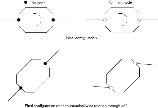The behavior of the two types of connections is illustrated in Figure 1, which shows an octagonal rigid body connected to two deformable shell elements through nodes at opposite ends subjected to an applied rotational velocity.

Figure 1. Rigid body with tie node and pin node connections.

The shell elements are shown with negligible bending in the figure above. When the nodes common to the rigid body and the shell elements are tie nodes, the rotation applied to the rigid body is transmitted directly to the shell elements. When the common nodes are pin nodes, the rigid body rotation is not transmitted directly to the shell elements, which can result in large relative motions between the rigid body and the adjacent shell structure.

To include elements in the rigid body definition, you specify the region of your model containing all the elements that are part of the rigid body. Elements in this region or nodes connected to the elements in this region cannot be part of any other rigid body. Table 1 lists the continuum, structural, and rigid element types that can be included in a rigid body.

The degrees of freedom active at the nodes of these elements depend on the element type (the same way they would if the elements were not included in the rigid body). If a connector element is part of a rigid body, the active degrees of freedom at the corresponding nodes further depend on the connection type. In addition, if connector elements that activate material flow degree of freedom at nodes are included in the rigid body, the material and flow through the rigid body as that degree of freedom is constrained to the motion of the rigid body.

The following elements cannot be declared as rigid:

• Acoustic elements
• Axisymmetric-asymmetric continuum and shell elements
• Coupled thermal-electrical elements
• Diffusive heat transfer/mass diffusion elements and forced convection/diffusion elements
• Eulerian elements
• Discrete elements
• Generalized plane strain elements
• Gasket elements with thickness-direction behavior
• Heat capacitance elements
• Inertial elements (mass and rotary inertia)
• Infinite elements
• Piezoelectric elements
• Special-purpose elements
• Substructures
• Thermal-electrical-structural elements
• User-defined elements

If elements of more than one type or section definition are part of a rigid body, the specified region will contain elements with different section definitions. When continuum or structural elements are assigned to a rigid body, they are no longer deformable and their motion is governed by the motion of the rigid body reference node. Element stiffness calculations are not performed for these elements, and they do not affect the global time increment in Abaqus/Explicit. However, the mass and inertia of the rigid body includes contributions from these elements as calculated from their section and material density definitions (see About the Element Library). Mass and rotary inertia elements, as well as point heat capacitance elements, should not be included in the specified region. Contributions to a rigid body from mass, rotary inertia, and heat capacitance elements are accounted for automatically when these elements are connected to nodes that are part of the rigid body.

A list of nodes that are part of a rigid body is generated automatically when you assign elements to a rigid body. The node list is constructed as a unique list including all the nodes that are connected to elements in the specified region. Nodes in this list cannot be part of any other rigid body. The type of each node, pin, or tie is determined by the type of elements on the rigid body to which it is connected. Shell, beam, pipe, and rigid beam elements generate tie nodes; solid, membrane, truss, and rigid (other than beam) elements generate pin nodes (see Table 1). For nodes that are connected to both elements that generate pin nodes and elements that generate tie nodes, the common node is defined as the tie type.

All elements that are part of a rigid body must be of like geometry. Therefore, elements contained in the specified region must be either planar, axisymmetric, or three-dimensional. The geometry of the elements determines the geometry of the rigid body as shown in Table 1.

RIGID BODY, REF NODE=n, ELSET=name

Interaction module: Create Constraint: Rigid body: Body (elements): Edit: select body regions

To assign nodes directly to a rigid body, you specify all the desired pin nodes and all the tie nodes separately. These nodes become part of the rigid body in addition to any nodes that have been generated from elements assigned to the rigid body. The following rules apply when assigning nodes directly to a rigid body:

• The rigid body reference node cannot be contained in either the set of pin nodes or the set of tie nodes.

• Nodes that are part of the set of pin nodes cannot also be contained in the set of tie nodes.

• Nodes that are contained in the set of pin nodes or the set of tie nodes cannot be part of any other rigid body definition.

• Nodes that are generated automatically from elements assigned to the rigid body that are also contained in the set of pin nodes are classified as pin nodes, regardless of their element connections.

• Nodes that are generated automatically from elements assigned to the rigid body that are also contained in the set of tie nodes are classified as tie nodes, regardless of their element connections.

The types of nodes generated by elements included in a rigid body can, therefore, be overridden by assigning the nodes directly to the rigid body, thereby allowing you greater flexibility to define a constraint with a rigid body by easily specifying the type of connection the rigid body makes with its attached deformable finite elements.

RIGID BODY, REF NODE=n, PIN NSET=name, TIE NSET=name

Interaction module: Create Constraint: Rigid body: Pin (nodes): Edit: select pin regions, and Tie (nodes): Edit: select tie regions

You can assign an analytical surface to a rigid body. The procedure for creating and naming an analytical rigid surface is described in Analytical Rigid Surface Definition. Only one analytical surface can be defined as part of the rigid body definition.

RIGID BODY, REF NODE=n or name, ANALYTICAL SURFACE=name

Interaction module: Create Constraint: Rigid body: Analytical Surface: Edit: select analytical surface regions

An Abaqus model can be defined in terms of an assembly of part instances (see Assembly Definition). A rigid body in such a model can be created from deformable elements at either the part level or the assembly level. In either case all node and element definitions must belong to one or more parts. If all nodes making up the rigid body belong to the same part, create a rigid part by defining the rigid body at the part level.

Multiple deformable part instances can be combined into a single rigid body by creating an assembly-level node or element set that spans the part instances, then defining the rigid body at the assembly level to refer to that set. The rigid body reference node can also be defined at the assembly level, if necessary.

In many cases it is desirable to model rigid components for which the mass, center of mass, and rotary inertia are not readily available. In Abaqus it is not necessary to define the mass and inertia properties of the rigid body directly. Instead, a finite element discretization can be used to model the rigid components, and Abaqus will automatically calculate the properties from the discretization. Rigid structures with one-dimensional rod or beam geometries can be modeled with beam or truss elements, structures containing two-dimensional surface geometries can be modeled with shell or membrane elements, and solid geometries can be modeled with solid elements. The mass contributions to the rigid body for each of these elements are based on that element's section properties (see About the Element Library) and the material density (see Density). Although both shell and membrane elements in a rigid body can yield similar mass contributions given similar section and density definitions, they will generate different node types (tie nodes for shells and pin nodes for membranes), which might affect the overall results. The same holds true for beam and truss elements.

In situations where one portion of a rigid component can be modeled with a finite element discretization but it is not convenient to do so for other portions, point mass and rotary inertia elements can be used to represent the mass distribution of these other portions. The mass, center of mass, and rotary inertia for the rigid body will then include the contributions from both the finite elements and the point mass and rotary inertia elements.

Abaqus uses the lumped mass formulation for low-order elements. As a consequence, the second mass moments of inertia can deviate from the theoretical values, especially for coarse meshes. This inaccuracy can be circumvented by adding point mass and rotary inertia elements with the correct inertia properties and eliminating the mass contribution from the solid elements. Alternatively, second-order elements could be used in Abaqus/Standard.

When the mass, center of mass, and rotary inertia properties of the actual rigid component are known or can be approximated, it is not necessary to use a finite element discretization or to use an array of point masses to generate the rigid body properties. You can assign these properties directly by locating the rigid body reference node at the center of mass (see Positioning the Reference Node at the Center of Mass) and by specifying the rigid body mass and rotary inertia at the reference node (see Point Masses and Rotary Inertia).

It might also be desirable to input mass properties directly at the center of mass but to specify boundary conditions at a location other than the center of mass. In this case you should place the rigid body reference node at the desired boundary condition location. In addition, you must define a tie node at the center of mass of the rigid body by correctly specifying its coordinates to coincide with the coordinates of the center of mass of the rigid body and then assigning it to a tie node set in the rigid body definition. You can then define the rigid body mass and rotary inertia at the tie node.

For most applications where mass properties are input directly, it might be necessary to assign additional elements or nodes to a rigid body so that the rigid body can interact with the rest of the model. For example, contact pair definitions could require rigid surfaces formed with element faces on the rigid body and additional pin or tie nodes might be necessary to provide the desired constraints with deformable elements attached to the rigid body. Abaqus will account for the mass and rotary inertia contributions from all elements on a rigid body; therefore, if you want to assign the rigid body mass properties directly, you should take care to ensure that contributions from other element types that are part of the rigid body do not affect the desired input mass properties. If rigid elements are part of the rigid body definition, you can set their mass contribution to zero by not specifying a density for these elements in the rigid body definition. If other element types are used to define the rigid body, you should set their density to zero.

A rigid body can undergo free rigid body motion in each of its active translational degrees of freedom, as well as each of its active rotational degrees of freedom.

Boundary conditions for rigid bodies should be defined as described in Boundary Conditions at the rigid body reference node. Reaction forces and moments can be recovered for all degrees of freedom that are constrained at the reference node. If a nodal transformation is defined at the rigid body reference node, boundary conditions are applied in the local system (see Transformed Coordinate Systems).

In Abaqus/Standard, if boundary conditions are applied to any nodes on a rigid body other than the rigid body reference node, Abaqus will attempt to transfer these boundary conditions to the reference node. If successful, you are warned that this transfer has taken place. Otherwise, an error message is produced (see Overconstraint Checks for more details).

In Abaqus/Explicit, if boundary conditions are applied to any nodes on a rigid body other than the rigid body reference node, these boundary conditions are ignored with the exception of the symmetry-type boundary conditions that can affect the contact logic at the perimeter of a surface in the Abaqus/Explicit contact pair algorithm (see Contact Formulations for Contact Pairs in Abaqus/Explicit and Common Difficulties Associated with Contact Modeling Using Contact Pairs in Abaqus/Explicit).

In Abaqus/Standard nodes on a rigid body, excluding the rigid body reference node, cannot be used in a multi-point constraint or linear constraint equation definition.

In Abaqus/Explicit a multi-point constraint or linear constraint equation can be defined for any node on a rigid body, including the reference node.

Connector elements can be used at any node of a rigid body, including the reference node, to define a connection between rigid bodies, between a rigid body and a deformable body, or from a rigid body to ground. Connector elements are convenient for providing multiple points of attachment on rigid bodies; modeling complex nonlinear kinematic constraints; specifying zero or nonzero boundary conditions at a point on a rigid body that is not the rigid body reference node; applying force actuation; and modeling discrete interactions, such as spring, dashpot, node-to-node contact, friction, locking mechanisms, and failure joints. Unlike multi-point constraints or linear constraint equations, connector elements retain degrees of freedom in the connection, thereby allowing output of information related to the connection (such as constraint forces and moments, relative displacements, velocities, accelerations, etc.). See Connector Elements for a detailed description of connector elements.

A rigid body with a planar geometry has three active degrees of freedom: 1, 2, and 6 ( $u_x$ , $u_y$ , and ${\varphi }_z$ ). Here, the x- and y-directions coincide with the global X- and Y-directions, respectively. If a nodal transformation is defined at the rigid body reference node, the x- and y-directions coincide with the user-defined local directions. The coordinate transformation defined at the reference node must be consistent with the geometry; the local directions must remain in the global X–Y plane. All nodes and elements that are part of a planar rigid body should lie in the global X–Y plane.

Planar rigid bodies should be connected only to planar deformable elements. To model the connection of a rigid component with a planar geometry to three-dimensional deformable elements, model the planar rigid component as a three-dimensional rigid body consisting of the appropriate three-dimensional elements.

A rigid body with an axisymmetric geometry has three active degrees of freedom in Abaqus: 1, 2, and 6 ( $u_r$ , $u_z$ , $\varphi$ ). Classical axisymmetric theory admits only one rigid body mode, which is displacement in the z-direction. To maximize the flexibility of using rigid bodies for axisymmetric analysis, Abaqus allows for three active degrees of freedom, although only the axial displacement is a rigid body mode.

The r- and z-directions coincide with the global X- and Y-directions, respectively. If a nodal transformation is defined at the rigid body reference node, the r- and z-directions coincide with the user-defined local directions. The coordinate transformation defined at the reference node must be consistent with the geometry; the local directions must remain in the global X–Y plane. All nodes and elements that are part of an axisymmetric rigid body should lie in the global X–Y plane.

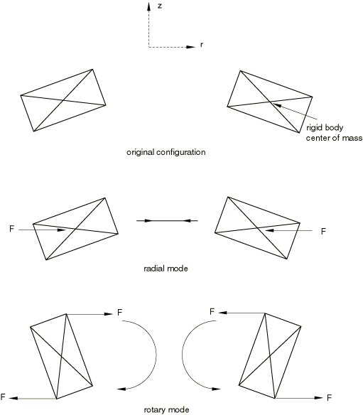
Translation in the r-direction is associated with a radial mode, and rotation in the r–z plane is associated with a rotary mode (see Figure 2). For an axisymmetric rigid body in Abaqus each of these modes develop no hoop stress, but mass and inertia computed for these degrees of freedom represent the modal mass associated with their modal motion. The mass properties for an axisymmetric rigid body are, therefore, calculated based on the initial configuration assuming the following:

• Point masses defined on nodes of the rigid body (see Point Masses) are assumed to account for the entire mass around the circumference of the body.

• Mass contributions from axisymmetric elements assigned to the rigid body include the integrated value around the circumference.

• The center of mass of the rigid body is located at the center of mass of the circumferential slice, as shown in Figure 2.

  Figure 2. Axisymmetric rigid body modes.
  
  

If the rigid body reference node is positioned at the center of mass, the reference node for an axisymmetric rigid body will, thus, be repositioned at the center of mass of the circumferential slice.

These assumptions are consistent with the manner in which Abaqus handles other axisymmetric features but are noted here because of the deviation from classical rigid body theory.

Axisymmetric rigid bodies should be connected only to axisymmetric deformable elements. To model the connection of a rigid component with an axisymmetric geometry to three-dimensional deformable elements, model the axisymmetric rigid component as a three-dimensional rigid body consisting of the appropriate three-dimensional elements.

A rigid body with a three-dimensional geometry has six active degrees of freedom: 1, 2, 3, 4, 5, and 6 ( $u_x$ , $u_y$ , $u_z$ , ${\varphi }_x$ , ${\varphi }_y$ , ${\varphi }_z$ ). Here, the x-, y-, and z-directions coincide with the global X-, Y- and Z-directions, respectively. If a nodal transformation is defined at the rigid body reference node, the x-, y-, and z-directions coincide with the user-defined local directions.

In general, three-dimensional rigid bodies will possess a full, nonisotropic inertia tensor and can behave in a nonintuitive manner when they are spun about an axis that is not one of the principal inertia axes. Classical phenomena of rigid body dynamics (for example, precession, gyroscopic moments, etc.) can be simulated using three-dimensional rigid bodies in Abaqus.

In most cases three-dimensional rigid bodies should be connected only to three-dimensional deformable elements. If it is physically relevant, a three-dimensional rigid body can be connected to two-dimensional plane stress, plane strain, or axisymmetric elements; however, you should always constrain the z-displacement, x-axis rotation, and y-axis rotation of the rigid body. 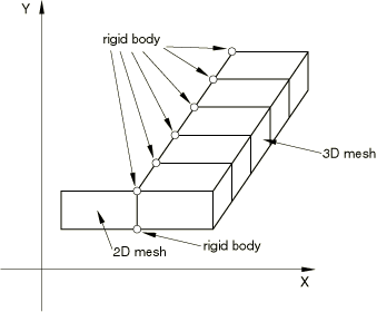The above procedure is useful when incorporating a two-dimensional plane strain approximation in one region of a model and a three-dimensional discretization in another. Rigid bodies can be used to constrain the two finite element geometries at their interface as shown in Figure 3. A unique rigid body should be used at each node in the plane along the interface to handle the constraint properly.

Figure 3. Rigid body nodes used to connect a two-dimensional and three-dimensional mesh.

Contact between rigid bodies is allowed if the secondary surface belongs to an elastic body that has been declared as rigid. In this case softened contact should be prescribed to avoid possible overconstraints.

Contact between two rigid surfaces defined using rigid elements is not allowed.

Rigid beams and trusses cannot be included in a contact pair definition because surfaces from beams and trusses can be node-based surfaces only. A node-based surface must be a secondary surface, and elements that are part of a rigid body should be part of the main surface in a contact pair.

Contact between two rigid surfaces can be modeled in Abaqus/Explicit only if the penalty contact pair algorithm or the general contact algorithm is used; kinematic contact pairs cannot be used for rigid-to-rigid contact. Therefore, when converting two deformable regions of a model to two distinct rigid bodies for the purpose of model development, any contact interaction definitions between these rigid bodies must use penalty contact pairs or general contact.

For rigid-to-rigid contact involving analytical rigid surfaces, at least one of the rigid surfaces must be formed by element faces since contact between two analytical rigid surfaces cannot be modeled in Abaqus.

The penalty contact pair algorithm, which introduces numerical softening to the contact enforcement through the use of penalty springs, or the general contact algorithm must be used for all contact interactions involving a rigid body if an equation constraint, a multi-point constraint, a tie constraint, or a connector element is defined for a node on the rigid body.

Rigid beams and trusses cannot be included in a kinematic contact pair definition because surfaces from beams and trusses can be node-based surfaces only. A node-based surface must be a secondary surface, and elements that are part of a rigid body must be part of the main surface in a kinematic contact pair.

When a rigid surface acts as a secondary surface in a penalty contact pair or in general contact, initial penetrations of the rigid secondary nodes into the main surface will not be corrected with strain-free corrections (see Contact Initialization for Contact Pairs in Abaqus/Explicit and Contact Initialization for General Contact in Abaqus/Explicit). For contact pairs any initial penetrations of this type might cause artificially large contact forces in the initial increments. For general contact these initial penetrations are stored as contact offsets.

The motion of the rigid body is entirely defined by the motion of its reference node; therefore, each tie node of the rigid body undergoes the same rotation as the reference node. The output of the rotation at the rigid body nodes is not available except at the reference node.