Thermal Contact Properties

Thermal Properties in a Contact Property Definition

You can include all the thermal properties discussed in this section—thermal contact conductance, gap radiation, and gap heat generation—in a contact property definition for both surface-based contact and element-based contact. All three types of thermal properties can be included in the same contact property definition. Nonzero default thermal properties (which you can override) include:

Contact conductance for touching surfaces: by default, a high value of thermal contact conductance is assigned across an interface with touching surfaces. The magnitude of this conductance is computed analogously to the default mechanical penalty stiffness to numerically approximate a condition of matched temperature across the interface without the risk of causing overconstraints or other numerical problems.
Dissipated energy at an interface: all dissipated energy at an interface is converted into heat by default for the gap heat generation mechanisms discussed in this section.

The thermal contact property model between two surfaces can also be completely defined through user subroutine UINTER, VUINTER, or VUINTERACTION (see User-Defined Interfacial Constitutive Behavior).

These thermal contact interaction models are intended for cases in which heat flow occurs between touching or nearby surfaces. Modeling thermal interactions over large distances with these models is often inaccurate and can significantly degrade performance.

Input File Usage

Use the following options for surface-based contact:

SURFACE INTERACTION, NAME=name
GAP CONDUCTANCE
GAP RADIATION
GAP HEAT GENERATION

Use the following options for element-based contact in Abaqus/Standard:

INTERFACE or GAP, ELSET=name
GAP CONDUCTANCE
GAP RADIATION
GAP HEAT GENERATION

Use the following option for user-defined, surface-based contact:

SURFACE INTERACTION, USER

Abaqus/CAE Usage

Interaction module: contact property editor: ThermalThermal Conductance, Heat Generation, and/or Radiation

Element-based contact and user-defined surface-based contact are not supported in Abaqus/CAE.

Contact Conductance between Surfaces

The conductive heat transfer between the contact surfaces is assumed to be defined by

q = k (θ_{A} - θ_{B}),

where q is the heat flux per unit area crossing the interface from point A on one surface to point B on the other,

θ_{A}

and

θ_{B}

are the temperatures of the points on the surfaces, and k is the thermal contact conductance. Point A is a node on the secondary surface; and point B is the location on the main surface contacting the secondary node or, if the surfaces are not in contact, the location on the main surface with a surface normal that intersects the secondary node.

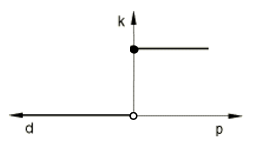
Common physical behavior is such that thermal conductance across an interface is much larger while surfaces are touching (“closed” contact status) than while separated (“open” contact status). By default, Abaqus assigns a large value for k to regions in contact (independent of the contact pressure, p) and assigns k=0 to regions not actively in contact (independent of the contact clearance distance, d), as shown in Figure 1.

For heat transfer or coupled thermal-electrical analyses, the contact pressure is always zero. Therefore, contact conductance at zero contact pressure is adopted for a closed initial contact status. When the contact status is open, a contact conductance value that is a function of clearance (if provided) or a zero value is chosen.

You can define k directly or, in Abaqus/Standard, in user subroutine GAPCON.

Modifying Contact Conductance

The default contact conductance (shown in Figure 1) differs if the contact status is closed or open, but it does not depend on the contact pressure or contact clearance distance. You can modify the contact conductance for closed and open contact regimes independently and introduce dependence of the contact conductance on contact pressure and contact clearance. When defining k directly, define:

k = k (d, p, \bar{θ}, \bar{| \dot{m} |}, {\bar{f}}_{γ}),

where

d: is the clearance between A and B,
p: is the contact pressure transmitted across the interface between A and B,
$\bar{θ} = \frac{1}{2} (θ_{A} + θ_{B})$: is the average of the surface temperatures at A and B,
$\bar{| \dot{m} |} = \frac{1}{2} ({| \dot{m} |}_{A} + {| \dot{m} |}_{B})$: is the average of the magnitudes of the mass flow rates per unit area of the contact surfaces at A and B (this variable is not considered in an Abaqus/Explicit analysis), and
${\bar{f}}_{γ} = \frac{1}{2} (f_{γ}^{A} + f_{γ}^{B})$: is the average of any predefined field variables at A and B.

Modifying Contact Conductance Where the Contact Status is Closed

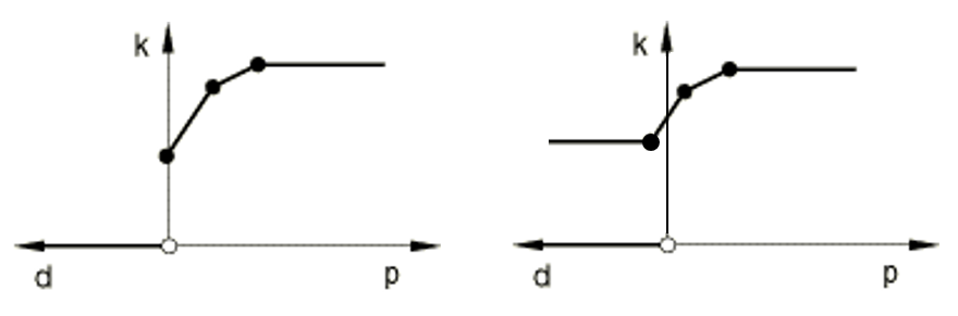
You can modify the contact conductance as a function of contact pressure where the contact status is closed, such as shown in Figure 2. When k is a function of contact pressure at the interface, the tabular data must start at zero contact pressure (or, in the case of contact that can support a tensile interface stress, the data point with the most negative pressure) and define k as p increases. The value of k remains constant for contact pressures beyond the range of data specified while contact is active. The contact conductance remains zero for separated surfaces not in contact for the examples shown in Figure 2. You can also modify the contact conductance for an open contact status as discussed in Modifying Contact Conductance Where the Contact Status is Open.

Input File Usage

GAP CONDUCTANCE, PRESSURE 
 $k$ , p,  $\bar{θ}$

Abaqus/CAE Usage

Interaction module: contact property editor: ThermalThermal Conductance: Definition: Tabular, Use only pressure-dependency data

Modifying Contact Conductance Where the Contact Status is Open

You can modify the contact conductance as a function of the contact clearance distance, d, where the contact status is open, such as shown in Figure 3. Tabular data associated with k dependence on d must start at zero clearance (closed gap) and define k as the clearance distance increases. You must define at least two k versus d data points to define k as a function of the clearance. The value of k immediately drops to zero for clearance distances larger than the last data point. Therefore, there is no heat conductance when the clearance distance is greater than the value corresponding to the last data point.

If you do not also define contact conductance as a function of contact pressure, the default value of k remains in effect where the contact status is closed, as shown in Figure 3. Figure 4 shows an example with the contact conductance specified as a function of contact pressure where the contact status is closed (as discussed in Modifying Contact Conductance Where the Contact Status is Closed) and as a function of contact clearance distance where the contact status is open.

Input File Usage

GAP CONDUCTANCE 
 $k$ , d,  $\bar{θ}$

Abaqus/CAE Usage

Interaction module: contact property editor: ThermalThermal Conductance: Definition: Tabular, Use only clearance-dependency data

Using Thermal Contact Conductance to Model Convective Heat Transfer from a Surface in Abaqus/Standard

Generally, mass flow rates are defined in Abaqus/Standard (see Forced Convection through the Mesh) only for nodes associated with forced convection elements. However, they can be defined for any node in a model. By using the dependence of k on the average mass flow rate at the interface (in addition to other dependencies), it is possible for the contact property definition to simulate convective heat transfer to the boundary layer between a solid and a moving fluid. If mass flow rates are given only for nodes on one side of the interface, which is typically the case when simulating convective heat transfer, the average mass flow rate $\bar{| \dot{m} |}$ used to define k is half the magnitude specified.

Input File Usage

GAP CONDUCTANCE 
k, d,  $\bar{θ}$ ,  $\bar{| \dot{m} |}$

Abaqus/CAE Usage

Interaction module: contact property editor: ThermalThermal Conductance: Definition: Tabular, Clearance Dependency and/or Pressure Dependency, toggle on Use mass flow rate-dependent data (Standard only)

Defining Thermal Contact Conductance as a Function of Predefined Field Variables

In addition to the dependencies mentioned previously, the thermal contact conductance can depend on any number of predefined field variables, ${\bar{f}}_{γ}$ . To make the thermal contact conductance depend on field variables, you must specify at least two data points for each field variable value.

Input File Usage

GAP CONDUCTANCE, DEPENDENCIES=n 
k, d,  $\bar{θ}$ ,  $\bar{| \dot{m} |}$ ,  ${\bar{f}}_{γ}$

Abaqus/CAE Usage

Interaction module: contact property editor: ThermalThermal Conductance: Definition: Tabular, Clearance Dependency and/or Pressure Dependency, Number of field variables: n

Defining the Thermal Contact Conductance Using User Subroutine GAPCON

In Abaqus/Standardk can be defined in user subroutine GAPCON. In this case there is greater flexibility in specifying the dependencies of k. It is no longer necessary to define k as a function of the average of the two surface's temperatures, mass flow rates, or field variables.

k = k (d, p, θ_{A}, θ_{B}, {| \dot{m} |}_{A}, {| \dot{m} |}_{B}, f_{γ}^{A}, f_{γ}^{B}) .

Input File Usage

GAP CONDUCTANCE, USER

Abaqus/CAE Usage

Interaction module: contact property editor: ThermalThermal Conductance: Definition: User-defined

Defining the Thermal Contact Conductance to Be Strongly Dependent on Temperature

If k depends strongly on temperature, the unsymmetric terms in the calculations start to become increasingly important in Abaqus/Standard. Using the unsymmetric matrix storage and solution scheme for the step might improve the convergence rate in the analysis (see Defining an Analysis).

Temperature and Field-Variable Dependence of Thermal Contact Conductance for Structural Elements

Temperature and field-variable distributions in beam and shell elements can generally include gradients through the cross-section of the element. Contact between these elements occurs at the reference surface; therefore, temperature and field-variable gradients in the element are not considered when determining thermal contact conductance, even in cases where the properties are also clearance dependent.

Thermal Contact Considerations in Abaqus/Explicit

Thermal contact conductance and gap radiation are enforced in Abaqus/Explicit with an explicit algorithm analogous to the penalty method for mechanical contact interaction. Therefore, thermal contact conductance and gap radiation can influence the stability condition; although in a fully coupled temperature-displacement analysis the mechanical portion of the system usually governs the overall stability condition (see Fully Coupled Thermal-Stress Analysis). Extremely large values of thermal contact conductance or gap radiation can result in a decrease in the stable time increment, which is accounted for by the automatic time incrementation algorithm in Abaqus/Explicit.

Gap heat generation is applied within whichever algorithm (kinematic or penalty) is used to enforce the mechanical contact constraints. Gap heat generation has no effect on the stable time increment.

Thermal contact fluxes might be inaccurate during increments in which mesh adaptivity occurs if the mechanical contact constraints are enforced kinematically, because mesh adjustments occur in Abaqus/Explicit between the determination of the mechanical contact state for kinematic contact and the calculation of thermal contact fluxes. For example, mesh adjustments for adaptivity might cause discontinuity in the contact pressure: for pressure-dependent thermal contact conductance, the thermal contact conductance coefficient is set based on the pressure determined by the kinematic contact algorithm prior to the mesh adjustment, even though the thermal contact flux is applied after the mesh adjustment. The significance of this inaccuracy on the solution depends on the size and frequency of the mesh adjustments and the degree of variation in the conduction coefficient. This inaccuracy can be avoided by enforcing the mechanical contact constraints with the penalty method.

Thermal contact properties cannot be specified for general contact involving edge-to-edge contact. Thermal contact involving shell elements defined in a contact pair definition conducts heat only through the temperature degrees of freedom on the bottom of the shell (NT11) regardless of the surface definition. This can produce nonphysical heat flow if the contact is on the top of the shell. In this case it is recommended that you use general contact as the proper degrees of freedom are used depending on which side of the shell is involved in contact.

Thermal interactions can occur between surfaces within the thermal contact distance associated with the thermal contact conductance or radiation model when another surface lies between them. This can result in unrealistic behavior for multiple layers of thin shells.

Modeling Radiation between Surfaces When the Gap Is Small

Abaqus assumes that radiative heat transfer between closely spaced contact surfaces occurs in the direction of the normal between the surfaces. In models using surface-based contact this normal corresponds to the main surface normal (see Contact Formulations in Abaqus/Standard, About Contact Pairs in Abaqus/Explicit, and About Surfaces). In models using the contact elements available in Abaqus/Standard the element's connectivity defines the normal direction.

The gap radiation functionality in Abaqus is intended for modeling radiation between surfaces across a narrow gap. A more general capability for modeling radiation is available in Abaqus/Standard (see Cavity Radiation in Abaqus/Standard).

Radiative heat transfer is defined as a function of clearance between the surfaces through the effective view factor. Abaqus maintains the radiative heat flux even when the surfaces are in contact. This causes only a minor inaccuracy since normally the heat flux from conduction is much larger than the radiative heat flux.

Abaqus defines the heat flow per unit surface area between corresponding points as

q = C [{(θ_{A} - θ^{Z})}^{4} - {(θ_{B} - θ^{Z})}^{4}],

where q is the heat flux per unit surface area crossing the gap at this point from surface A to surface B,

θ_{A}

and

θ_{B}

are the temperatures of the two surfaces,

θ^{Z}

is the absolute zero on the temperature scale being used, and the coefficient C is given by

C = \frac{F σ}{1 / ϵ_{A} + 1 / ϵ_{B} - 1},

where

σ

is the Stefan-Boltzmann constant,

ϵ_{A}

and

ϵ_{B}

are the surface emissivities, and F is the effective view factor, which corresponds to viewing the main surface from the secondary surface.

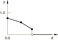
The view factor F must be defined as a function of the clearance, d, and should have a value between 0.0 and 1.0. The expression above accurately represents the radiation heat exchange between two infinite plates that are close to each other, in which case the effective view factor, F equals 1.0. In all other cases, the effective view factor serves as a scaling factor used to approximate the radiation heat exchange between the two finite surfaces. At least two pairs of $F - d$ points are required to define the view factor, and the tabular data must start at zero clearance (closed gap) and define the view factor as the clearance increases. The value of F drops to zero immediately after the last data point, so there is no radiative heat transfer when the clearance is greater than the value corresponding to the last data point (see Figure 5).

Input File Usage

GAP RADIATION 
 $ϵ_{A}$ ,  $ϵ_{B}$  
 $F_{0}$ ,  $0.$  
 $F_{1}$ ,  $d_{1}$  
…

Abaqus/CAE Usage

Interaction module: contact property editor: ThermalRadiation: Emissivity of secondary surface:  $ϵ_{A}$ , Emissivity of main surface:  $ϵ_{B}$ , View factor and Clearance

Specifying the Value of Absolute Zero

You must specify the value of $θ^{Z}$ .

Input File Usage

PHYSICAL CONSTANTS, ABSOLUTE ZERO= $θ^{Z}$

Abaqus/CAE Usage

Any module: ModelEdit Attributesmodel_name: Absolute zero temperature:  $θ^{Z}$

Specifying the Stefan-Boltzmann Constant

You must specify the Stefan-Boltzmann constant, $σ$ .

Input File Usage

PHYSICAL CONSTANTS, STEFAN BOLTZMANN= $σ$

Abaqus/CAE Usage

Any module: ModelEdit Attributesmodel_name: Stefan-Boltzmann constant:  $σ$

Improving Convergence in Abaqus/Standard

Since the heat flux due to radiation is a strongly nonlinear function of the temperature, the radiation equations are strongly nonsymmetric and using the unsymmetric matrix storage and solution scheme for the step might improve the convergence rate in Abaqus/Standard (see Defining an Analysis).

Modeling Heat Generated by Nonthermal Surface Interactions

In fully coupled temperature-displacement, fully coupled thermal-electrical-structural, or coupled thermal-electrical simulations, Abaqus allows for heat generation due to the dissipation of energy created by the mechanical or electrical interaction of contacting surfaces. The source of the heat in a fully coupled temperature-displacement analysis and a fully coupled thermal-electrical-structural analysis is frictional sliding; the source in a coupled thermal-electrical and a fully coupled thermal-electrical-structural analysis simulation is the flow of electrical current across the interface surfaces. By default, Abaqus releases all of the dissipated energy as heat between the surfaces and distributes it equally between the two interacting surfaces.

You can specify the fraction of dissipated energy converted into heat, $η$ (default is 1.0), and the weighting factor, f (default is 0.5), for distribution of the heat between the interacting surfaces. $η$ often includes a factor to convert mechanical energy into thermal energy.

f = 1.0 indicates that all of the generated heat flows into the first (secondary) surface of the contact pair. f = 0.0 indicates that all of the generated heat flows into the opposite (main) surface. Unless valid experimental data suggest otherwise, it is best to assume the default value of f = 0.5 because this value evenly distributes the generated heat between the surfaces. Due to surfaces often acting in both secondary and main roles for general contact, the results can be difficult to interpret when f is different than 0.5. In this case you should use the pure main-secondary formulation.

If user subroutine UINTER, VUINTER, or VUINTERACTION is used to define the interfacial constitutive behavior, all gap heat generation effects are turned off; you must supply an additional heat flux in the user subroutine to model these effects.

Input File Usage

GAP HEAT GENERATION 
 $η$ , f

Abaqus/CAE Usage

Interaction module: contact property editor: ThermalHeat Generation: Specify:  $η$  and f

Heat Generated due to Frictional Sliding

In coupled thermomechanical and coupled thermal-electrical-structural surface interactions, the rate of frictional energy dissipation is given by

P_{f r} = τ \cdot \dot{γ},

where

τ

is the frictional stress and

\dot{γ}

is the slip rate. The amount of this energy released as heat on each surface is assumed to be

q_{A} = f η P_{f r} and q_{B} = (1 - f) η P_{f r},

where

η

and f are defined above. The heat flux into the secondary surface is

q_{A}

, and the heat into the main surface is

q_{B}

.

Heat Generated due to Flow of Electrical Current in Abaqus/Standard

In a coupled thermal-electrical analysis (see Coupled Thermal-Electrical Analysis) and a fully coupled thermal-electrical-structural analysis (see Fully Coupled Thermal-Electrical-Structural Analysis), the rate of electrical energy dissipated by electric current flowing across the interface is

P_{e c} = J (φ_{A} - φ_{B}),

where J is the electrical current density and

φ_{A}

and

φ_{B}

are the electrical potentials on the two surfaces. The amount of this energy released as heat on each of the interface surfaces is assumed to be

q_{A} = f η P_{e c} and q_{B} = (1 - f) η P_{e c},

where

η

and f are defined in the same way as for frictional dissipation. Again, the heat flux into the secondary surface is

q_{A}

, and the heat into the main surface is

q_{B}

.

Surface-Based Interaction Variables for Thermal Contact Property Models

Abaqus provides many output variables related to the thermal interaction of surfaces. In Abaqus/Standard the values of these variables are always given at the nodes of the secondary surface. In Abaqus/Explicit these variables can be output for main and secondary surfaces, although they are not available for analytical surfaces. The variables are available only for simulations that use surface-based contact definitions. They can be requested as surface output to the data, results, or output database files (see Surface Output from Abaqus/Standard and Writing Surface Output to the Output Database for details).

Surface-Based Interaction Variables for Heat Fluxes

The following variables are available for any simulation in which heat transfer can occur (fully coupled temperature-displacement, fully coupled thermal-electrical-structural, coupled thermal-electrical, or pure heat transfer analyses):

HFL: Heat flux per unit area leaving the surface.
HFLA: HFL multiplied by the nodal area.
HTL: Time integrated HFL.
HTLA: Time integrated HFLA.

Abaqus/Standard provides all of these variables by default whenever surface output is requested to the data or results file and thermal surface interactions are present.

These variables can also be displayed in contour plots in the Visualization module of Abaqus/CAE (Abaqus/Viewer).

Surface-Based Interaction Variables for Heat Generated by Frictional Sliding

The following variables are available for fully coupled temperature-displacement simulations in which there is frictional interaction between contacting surfaces or user subroutine UINTER, VUINTER, or VUINTERACTION is used:

SFDR: Heat flux per unit area entering the surface due to frictional dissipation (includes heat flux to both surfaces, $q_{A}$ and $q_{B}$ ). When user subroutine UINTER, VUINTER, or VUINTERACTION is used to define the interfacial thermal constitutive behavior, this quantity represents the heat flux resulting from the total energy dissipation due to friction and other dissipative effects. The effects of gap heat generation are turned off.
SFDRA: SFDR multiplied by the nodal area.
SFDRT: Time integrated SFDR.
SFDRTA: Time integrated SFDRA.
WEIGHT: Weighting factor, f, for heat flux distribution between the surfaces (available only in Abaqus/Standard; not available when the constitutive behavior of the interface is defined using user subroutine UINTER).

Abaqus/Standard does not provide these variables by default when surface output is requested to the data or results file; you must specify the variable identifiers.

Contour plots of these variables can also be created in the Visualization module of Abaqus/CAE (Abaqus/Viewer).

Surface-Based Interaction Variables for Heat Generated by Electrical Currents

The following variables are available for any coupled thermal-electrical and any fully coupled thermal-electrical-structural simulation:

SJD: Heat flux per unit area generated by the electrical current, includes heat flux to both surfaces ( $q_{A}$ and $q_{B}$ ).
SJDA: SJD multiplied by area.
SJDT: Time integrated SJD.
SJDTA: Time integrated SJDA.
WEIGHT: Weighting factor, f, for heat flux distribution between the surfaces.

Abaqus/Standard does not provide these variables by default when surface output is requested to the data or results file; you must specify the variable identifiers.

Contour plots of these variables can also be plotted in the Visualization module of Abaqus/CAE (Abaqus/Viewer).

Surface-Based Interaction Variables for Heat Generated by Electrical Contact Conductance

SJDE: Heat flux per unit area due to electrical current in electrolyte.
SJDEA: SJDE multiplied by the nodal area.
SJDET: Time integrated SJDE.
SJDETA: Time integrated SJDEA.

Thermal Interaction Variables for Thermal Gap Elements

Abaqus/Standard provides the heat flux per unit area across the thermal gap elements as output. Request element output of the variable identifier HFL to the data, results, or output database file (see Element Output and Writing Element Output to the Output Database for details). The only nonzero component is HFL1: there is no heat flux tangential to the interface defined by the gap element. A positive value of HFL1 indicates heat flowing in the direction of the normal to the main surface side of the element (see Gap Contact Elements for the definition of this normal for DGAP elements).

Contours of the heat flux across the thermal contact elements can be plotted using Abaqus/CAE.

Thermal Interactions Involving Rigid Bodies

Various factors to consider when modeling thermal interactions involving rigid bodies are discussed in Rigid Body Definition. For example, Abaqus/Standard does not allow modeling of thermal interactions with analytical rigid surfaces.

Modeling Thermal Interactions with Node-Based Surfaces

The following limitations apply to fully coupled thermal-electrical-structural and fully coupled thermal-stress analyses (see Fully Coupled Thermal-Stress Analysis) in Abaqus/Standard:

No heat flow occurs across a contact pair involving a node-based surface.
No heat generation occurs for a contact pair involving a node-based surface.

These limitations do not apply to Abaqus/Explicit and do not apply to other analysis types involving thermal interactions in Abaqus/Standard (see About Heat Transfer Analysis Procedures).

However, when allowed, use node-based surfaces for thermal interactions with caution: Abaqus calculates the thermal interaction between bodies in terms of nodal heat fluxes that must consider the actual contact surface area associated with each node. In Abaqus/Standard this area must be specified precisely for each node in the node-based surface to calculate the correct heat fluxes; in Abaqus/Explicit a unit area is assigned to each node of a node-based surface (see Node-Based Surface Definition).

Thermal Interactions between Surfaces with Nodes Containing Multiple Temperature Degrees of Freedom

When the surfaces involved in a thermal interaction are defined on shell elements that have multiple temperature degrees of freedom at each node, the choice of the temperature degree of freedom at a given node for the thermal interaction depends on how the surface is defined. For an element-based surface the temperature degree of freedom closest to the surface is chosen; that is, the first temperature degree of freedom at the node for the bottom surface and the last temperature degree of freedom at the node for the top surface. For a node-based surface, the first temperature degree of freedom at the node is always chosen for a thermal interaction.