Modified Riks algorithm

Let $P^N\mathit{ }(N=1,2,\mathrm{\dots }$ = the degrees of freedom of the model) be the loading pattern, as defined with one or more of the loading options in Abaqus. Let $\lambda$ be the load magnitude parameter, so at any time the actual load state is $\lambda P^N$, and let $u^N$ be the displacements at that time.

The solution space is scaled to make the dimensions approximately the same magnitude on each axis. In Abaqus this is done by measuring the maximum absolute value of all displacement variables, $\overline{u}$, in the initial (linear) iteration. We also define $\overline{P}={\left(P^N{P}^N\right)}^{\frac{1}{2}}$. The scaled space is then spanned by

• load $=\lambda {\tilde{P}}^N,{\tilde{P}}^N=P^N/\overline{P}$,

• displacements $={\tilde{u}}^N=(u^N/\overline{u});$

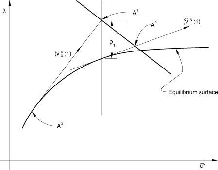
and the solution path is then the continuous set of equilibrium points described by the vector $\left({\tilde{u}}^N; \lambda \right)$ in this scaled space. All components of this vector will be of order unity. The algorithm is shown in Figure 2 and is described below.

Figure 2. Modified Riks algorithm.

Suppose the solution has been developed to the point $A^o=\left({\tilde{u}}_o^N;{\lambda }_o\right)$. The tangent stiffness, $K_o^{NM}$, is formed, and we solve

The increment size $(A^o\text{ to }{A}^1$ in Figure 2) is chosen from a specified path length, $\mathrm{\Delta }l$, in the solution space, so that

and, hence,

(here ${\tilde{v}}_o^N$ is $v_o^N$ scaled by $\overline{u}$). The value $\mathrm{\Delta }l$ is initially suggested by the user and is adjusted by the Abaqus/Standard automatic load incrementation algorithm for static problems, based on the convergence rate. The sign of $\mathrm{\Delta }{\lambda }_o$—the direction of response along the tangent line—is chosen so that the dot product of $\mathrm{\Delta }{\lambda }_o\left({\tilde{v}}_o^N;\mathrm{\hspace{0.25em}1}\right)$ on the solution to the previous increment, $\left(\mathrm{\Delta }{\tilde{u}}_{-1}^N;\hspace{1em}\mathrm{\Delta }{\lambda }_{-1}\right)$, is positive:

that is

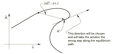
It is possible that in some cases, where the response shows very high curvature in the $\left({\tilde{u}}^N;\lambda \right)$ space, this criterion will cause the wrong sign to be chosen—see, for example, Figure 3.

Figure 3. Example of incorrect choice of sign for $\mathrm{\Delta }\lambda$.

The wrong sign is rarely chosen in practical cases, unless the increment size is too large or the solution bifurcates sharply. To check for such cases is computationally expensive: one approach would be for the solution to be found at ${\lambda }_o-\epsilon \mathrm{\Delta }{\lambda }_{-1},\mathrm{\hspace{0.25em}0}<\epsilon \ll 1$, so that we obtain a vector that gives a close approximation of the directed tangent at $A^o$. Because the case is so rare, such a check is not included, and the simple dot product given above is used alone to determine the sign of $\mathrm{\Delta }{\lambda }^o$. Thus, we have now found the point $A^1\left({\tilde{u}}_o^N+\mathrm{\Delta }{\lambda }_o{\tilde{v}}_o^N;{\lambda }_o+\mathrm{\Delta }{\lambda }_o\right)$ in Figure 2. The solution is now corrected onto the equilibrium path in the plane passing through $A^1$ and orthogonal to $\left({\tilde{v}}_o^N;1\right)$, by the following iterative algorithm.

• Initialize: $\mathrm{\Delta }{\lambda }_i=\mathrm{\Delta }{\lambda }_o,\mathrm{\Delta }{u}_i^N=\mathrm{\Delta }{\lambda }_0{v}_o^N$

• For $i=$ iteration $(i=1,\mathrm{\hspace{0.25em}2},\mathrm{\hspace{0.25em}3},\mathrm{etc}.)$:

  1. Form $I^N, K^{NM},$ the internal (stress) forces at the nodes,

     $$I^N={\int }_V{\mathit{\beta }}^N:\mathit{\sigma }dV,\text{ and }{K}^{NM}=\frac{\partial I^N}{\partial u^M},$$

     at the state $\left(u_o^N+\mathrm{\Delta }{u}_i^N; {\lambda }_o+\mathrm{\Delta }{\lambda }_i\right)$—that is, at $A^i$ in Figure 2.

  2. Check equilibrium:

     $$R_i^N=\left({\lambda }_o+\mathrm{\Delta }{\lambda }_i\right)P^N-I^N.$$

     If all the entries in $R_i^N$ are sufficiently small, the increment has converged. If not, we proceed.

  3. Solve:

     $$K^{NM}\left\{v_i^M;c_i^M\right\}=\left\{P^N;R_i^N\right\}.$$

     That is, we solve simultaneously with two load vectors, $P^N$ and $R^N$, and obtain two displacement vectors, $v_i^N$ and $c_i^N$.

  4. Now scale the vector $\left({\tilde{v}}_i^N;1\right)$, and add it to $\left({\tilde{c}}_i^N;{\rho }_i\right)$ where ${\rho }_i=R_i^N{P}^N/{\overline{P}}^2$ is the projection of the scaled residuals onto ${\tilde{P}}^N$ so that we move from $A^i$ to $A^{i+1}$ in the plane orthogonal to $\left({\tilde{v}}_o^N;1\right)$—see Figure 2. This gives the equation

     $$\left\{\left(0;-{\rho }_i\right)+\left({\tilde{c}}_i^N;{\rho }_i\right)+\mu \left({\tilde{v}}_i^N;1\right)\right\}:\left({\tilde{v}}_o^N;1\right)=0,$$

     which simplifies to give

     $$\mu =-\frac{{\tilde{c}}_i^N{\tilde{v}}_o^N}{{\tilde{v}}_i^N{\tilde{v}}_o^N+1},$$

     and the solution point is now $A^i$:

     $$\left(u_o^N+\mathrm{\Delta }{u}_i^N+c_i^N+\mu v_i^N;{\lambda }_o+\mathrm{\Delta }{\lambda }_i+\mu \right).$$

  5. Update for the next iteration,

     $$\begin{array}{cc}\hfill \mathrm{\Delta }{u}_{i+1}^N& =\mathrm{\Delta }{u}_i^N+c_i^N+\mu v_i^N\hfill \\ \hfill \mathrm{\Delta }{\lambda }_{i+1}& =\mathrm{\Delta }{\lambda }_i+\mu \hfill \\ \hfill i& =i+1,\hfill \end{array}$$

     and return to (a) above for the next iteration.

The implementation in Abaqus/Standard includes the additional update after each iteration:

This causes the equilibrium search to be orthogonal to the last tangent, rather than to the tangent at the beginning of the increment. The main motivation for this additional modification comes from the use of the method in plasticity problems, where the first iteration of each increment uses the elastic material stiffness to establish the direction of straining and so provides a stiffness that is not representative of the tangent to the equilibrium path if active plasticity is occurring.

The total path length traversed is determined by the load magnitudes supplied by the user on the loading options; while the number of increments is determined by the user-specified time increment data, assisted by Abaqus/Standard's automatic incrementation scheme if that is chosen.