This example examines the debonding behavior of a double cantilever beam.
The following Abaqus features are demonstrated:
predicting debond growth in a double cantilever beam
(DCB) using crack propagation analysis with the VCCT fracture criterion, the PRX-VCCT fracture criterion, cohesive elements, and surface-based cohesive behavior in Abaqus/Standard;
demonstrating the use of contact clearance assignment between surfaces with the VCCT fracture criterion and surface-based cohesive behavior in Abaqus/Explicit to predict debond growth;
restricting delamination growth and predicting the onset of debonding in models without a
predefined crack tip using cohesive elements to supplement the VCCT fracture criterion for modeling the Z-pins and stitches that are commonly used in
aerospace applications; and
predicting progressive delamination growth at the interface in a double cantilever beam
subjected to subcritical cyclic loading using the fatigue crack growth criterion based on
the Paris law.
This example examines the debonding behavior of a double cantilever beam. Debond onset and
growth are predicted for matched meshes in both Abaqus/Standard and Abaqus/Explicit and mismatched meshes in Abaqus/Standard. Different mesh discretizations are also used to investigate their effects on the
debonding behavior. The results from Abaqus/Standard are compared with the results obtained using the VCCT-based fracture interface elements in Mabson (2003), as well as the results predicted by
theory. The results predicted using VCCT, cohesive elements, and surface-based cohesive behavior in Abaqus/Standard are also compared. In addition, the results predicted by using the PRX-VCCT fracture criterion are compared with the results using the traditional VCCT fracture criterion.
The debonding behavior can also be studied by using the VCCT capability in Abaqus/Explicit. The model used in Abaqus/Explicit is constructed to achieve quasi-static behavior that allows the results obtained to be
comparable with those generated using VCCT in Abaqus/Standard.
The same model is analyzed in Abaqus/Standard using the fatigue crack growth criterion to assess the fatigue life when the model is
subjected to subcritical cyclic loading. The onset and delamination growth are characterized
using the Paris law, which relates the relative fracture energy release rate to the crack
growth rate. The fracture energy release rate at the crack tip is calculated based on the
VCCT technique. The results from Abaqus are compared with those predicted by the theory in Tada (1985).
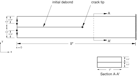
Geometry
The double cantilever beam in this example has a span of 9.0 in (228.6 mm) with a
rectangular cross-section of 1.0 in (25.4 mm) wide × 0.4 in (10.2 mm) deep, as shown in
Figure 1.
Boundary conditions and loading
One end of the beam is fixed, and the displacements are applied at the other end, as
shown in Figure 1. The
maximum displacement is set equal to 0.16 in (4.1 mm) in the monotonic loading cases. In
the fatigue crack growth analysis a cyclic displacement loading with a peak value of 0.05
in (1.3 mm) is specified.
Abaqus modeling approaches and simulation techniques
This example includes several two-dimensional models and one three-dimensional model.
Summary of analysis cases
Case 1
Prediction using matched and mismatched meshes for the
two-dimensional DCB model.
Case 2
Comparison using different mesh discretizations for the
two-dimensional DCB model.
Case 3
Theoretical and VCCT response prediction for the three-dimensional
DCB model.
Case 4
Using cohesive elements with VCCT debond to model crack initiation.
Case 5
Using cohesive elements with VCCT debond to model Z-pins and stitches.
Case 6
Fatigue crack growth prediction with the direct cyclic
approach, general fatigue crack growth approach, and simplified fatigue crack
growth approach using the same model as in Case 1.
Case 7
Fatigue crack growth prediction with the direct cyclic
approach using the same model as in Case 3.
Case 8
Comparison of the results obtained using VCCT, PRX-VCCT, cohesive elements, and cohesive behavior.
Case 9
Using cohesive behavior with VCCT in Abaqus/Explicit to model crack initiation. The model is identical to the model in Case 3.
Analysis Types
Static stress analyses are performed for Cases 1–8. Dynamic analysis is used for Case 9.
Case 1 Prediction using matched and mismatched meshes for the two-dimensional
DCB model
This case verifies that the simulation results agree with the experimental results and
compares the accuracy of the results obtained using matched and mismatched meshes.
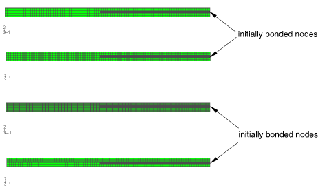
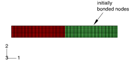
Mesh design
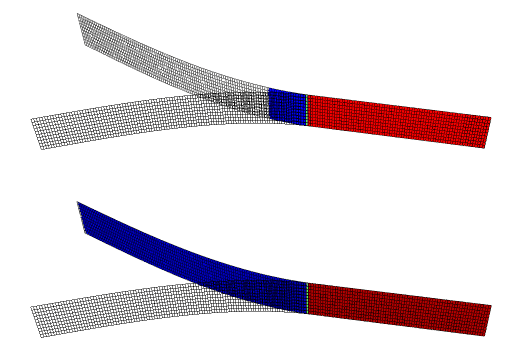
Four CPE4 elements are used to model the
thickness of each half of the beam. The top and bottom figures in Figure 2
show the configurations of undeformed meshes used here with the initially bonded nodes.
The model at the top has matched meshes with 90 × 4 meshes for each half of the
DCB, while the model at the bottom has mismatched meshes
with 90 × 4 meshes for the lower half and 85 × 4 meshes for the upper half of the
DCB.
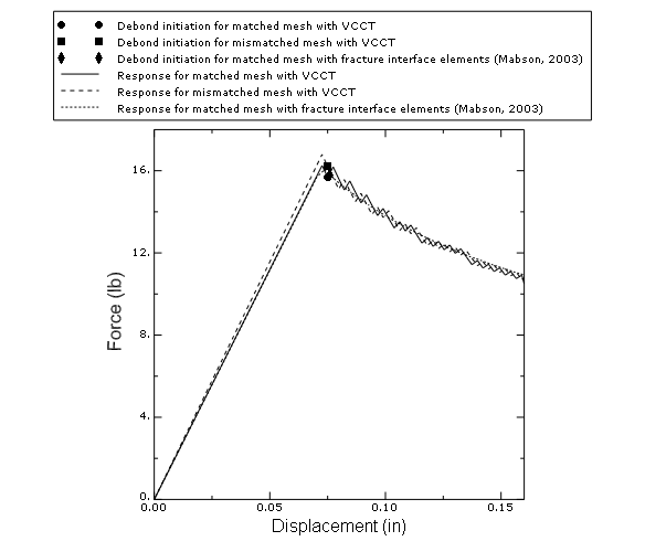
Results and discussion
The VCCT debond approach in Abaqus predicts the onset of debonding for both the matched and mismatched meshes accurately
within 3% of the prediction by the fracture interface elements, as shown in Figure 3.
Figure 3 also shows the growth prediction calculated by the VCCT debond approach.
Case 2 Comparison using different mesh discretizations for the two-dimensional
DCB model
This case shows the effect of mesh refinement on the response.
Mesh design
Four CPE4 elements are used to model the
thickness of each half of the beam, the same as in Case 1. The following mesh
discretizations are used along the span of the beam:
Matched mesh with 90 × 4 mesh for each half of the
DCB.
Matched mesh with 180 × 4 mesh for each half of the
DCB.
Matched mesh with 360 × 4 mesh for each half of the
DCB.
The meshes are displayed in Figure 2
(first three models).
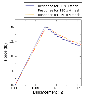
Results and discussion
Figure 4
shows the response for different mesh discretizations of the two-dimensional model of the
double cantilever beam and clearly illustrates the convergence of the response to the same
solution with mesh refinement. The maximum energy release rate cutback tolerance is set to
the default value of 0.2 in the input file provided for the two-dimensional model
(dcb_vcct_2d_1.inp). However, to eliminate factors other than mesh
size from the results shown in Figure 4,
the comparisons were run with the cutback tolerance reduced to 0.1.
Case 3 Theoretical and VCCT response prediction for the three-dimensional DCB
model
This case compares the three-dimensional results of Abaqus with the theoretical prediction.
Mesh design
The three-dimensional undeformed mesh and the initially bonded nodes are shown in Figure 5.
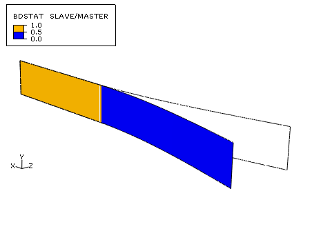
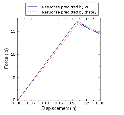
Results and discussion
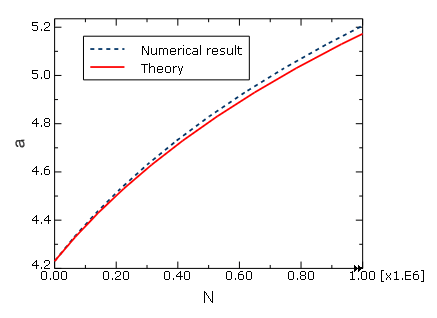
Figure 6
shows a contour plot of the solution-dependent state variable
BDSTAT for the three-dimensional model
of the double cantilever beam. The debond growth is shown on the right side of the model.
The response predicted by the VCCT debond approach in Abaqus after the onset of debonding closely matches the theoretical results for the
three-dimensional model of the double cantilever beam, as shown in Figure 7.
Case 4 Using cohesive elements with VCCT debond to model crack initiation
This case demonstrates how cohesive elements are used to initiate debond growth in a
two-dimensional VCCT model.
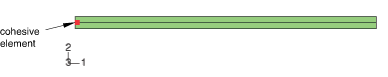
Mesh design
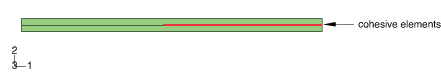
A zero-thickness cohesive element (shown in Figure 8)
is added at x = 0 at the interface between the two halves of the
DCB. The cohesive element bonds the nodes at
x = 0 at the contact interface. All the remaining nodes along the
contact interface are initially bonded (see Defining Initially Bonded Crack Surfaces in Abaqus/Standard).
Materials
The cohesive element properties are chosen such that the energy required for its complete
failure equals the fracture toughness of the interface. A damage initiation criterion is
specified for the cohesive element.
Case 5 Using cohesive elements with VCCT debond to model Z-pins and stitches
Z-pins and stitches are additional reinforcements used at the bonded interface to retard
the delamination growth. These can be modeled using zero-thickness cohesive elements at the
debond interface with the appropriate material and damage initiation and damage evolution
characteristics of the reinforcement. In the DCB model the
nodes at the interface (shown in Figure 9) are
initially bonded (see Defining Initially Bonded Crack Surfaces in Abaqus/Standard). In addition, a
layer of cohesive elements is defined at the interface using the initially bonded nodes to
represent the Z-pins and stitches.
Case 6 Fatigue prediction using the same model as in Case 1
This case verifies that delamination growth in a two-dimensional
DCB model subjected to subcritical cyclic loading can be
predicted using the fatigue crack growth criterion. Three different approaches are used in
this case: the direct cyclic approach, the general fatigue crack growth approach, and the
simplified fatigue crack growth approach. The simulation results are compared with the
theoretical results.
Mesh design
The model has matched meshes the same as in Case 1 (model at the top of Figure 2).
Results and discussion
The results in terms of crack length versus the cycle number obtained using the direct
cyclic approach in Abaqus are compared with the theoretical results in Figure 10.
Reasonably good agreement is obtained. Similarly, good results are obtained when using the
general and the simplified fatigue crack growth approaches.
Case 7 Fatigue prediction using the same model as in Case 3
This case verifies that delamination growth in a three-dimensional
DCB model subjected to subcritical cyclic loading can be
predicted using the fatigue crack growth criterion with the direct cyclic approach. The
simulation results are compared with the theoretical results.
Mesh design
The mesh design is the same as in Case 3 (Figure 5).
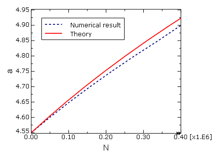
Results and discussion
The results in terms of crack length versus the cycle number obtained using the fatigue
crack growth criterion in Abaqus are compared with the theoretical results in Figure 11.
Reasonably good agreement is obtained.
Case 8 Comparison of the results obtained using VCCT, PRX-VCCT, cohesive elements, and cohesive behavior
This case compares the results obtained using VCCT, PRX-VCCT, cohesive elements, and surface-based cohesive behavior for both the two- and
three-dimensional DCB models.
Mesh design
For the two-dimensional model, four CPE4
elements are used to model the thickness of each half of the beam. The model at the top of
Figure 2
shows the configurations of undeformed meshes used here with the initially bonded nodes.
The model has matched meshes with 90 × 4 meshes for each half of the
DCB.
The three-dimensional undeformed mesh and the initially bonded nodes are shown in Figure 5.
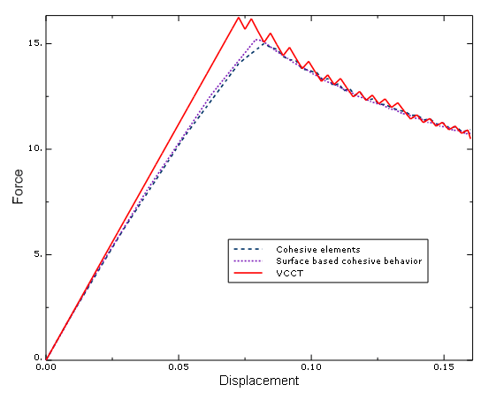
Results and discussion
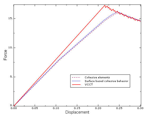
Figure 12
compares the results obtained using VCCT, cohesive elements, and surface-based cohesive behavior for the two-dimensional
DCB model. Figure 13
shows a similar comparison for the three-dimensional DCB
model. All of the methods predicted nearly the same debond growth after debond onset. But
the responses predicted using cohesive elements or surface-based cohesive behavior are not
strictly linear before debond onset, as compared with the linear behavior predicted by the
VCCT debond approach. This is not surprising since the secondary nodes for the model using
the VCCT debond approach are released one after another, while all the secondary nodes for the
models using cohesive elements or surface-based cohesive behavior debond simultaneously.
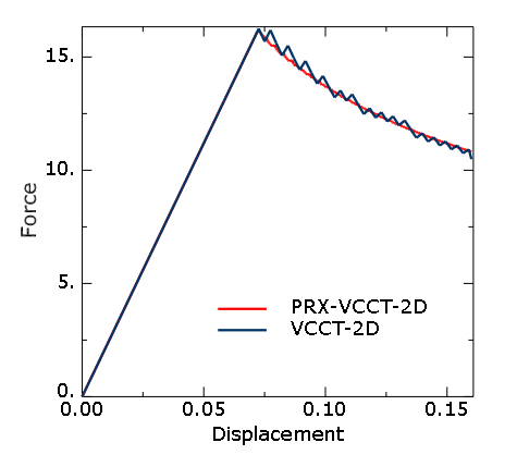
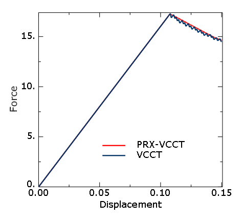
Similar comparisons have been made between VCCT and PRX-VCCT. Figure 14 shows the results for the two-dimensional model, while Figure 15 shows the results for the three-dimensional model. The loading curves using PRX-VCCT are much smoother than the ones using VCCT.
Case 9 Using VCCT in Abaqus/Explicit to model crack initiation
This case verifies that delamination growth in a three-dimensional
DCB model can be predicted using the VCCT capability in Abaqus/Explicit. The simulation results are compared with Abaqus/StandardVCCT results.
Mesh design
The mesh design is the same as in Case 3 (Figure 5).
Results and discussion
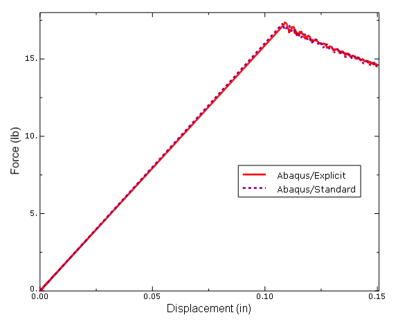
The debond states obtained from the Abaqus/Explicit and Abaqus/Standard analyses match very well, as depicted in Figure 16. The measured reaction forces from the Abaqus/Explicit analysis compare extremely well with those from Abaqus/Standard, as shown in Figure 17. The
debonding time, displacement, and energy release rate are highly consistent between both
analyses.
Abaqus/Explicit three-dimensional model with matched meshes.
References
Mabson, G, “Fracture Interface Elements,” 46th
PMC General Session of Mil-17 (Composites Materials
Handbook) Organization, Charleston, SC, 2003.
Tada, H, “The Stress Analysis of Cracks
Handbook,” Paris Productions Incorporated, 1985.
Figures
Figure 1. The double cantilever beam (DCB) model. Figure 2. Mesh configurations for the two-dimensional DCB
model. Figure 3. Debond onset and growth prediction for matched and mismatched meshes for the
two-dimensional DCB model. Figure 4. Response for different mesh discretizations of the two-dimensional
DCB model. Figure 5. Mesh configuration for the three-dimensional DCB
model. Figure 6. Debond growth for the three-dimensional DCB
model. Figure 7. Theoretical and VCCT in Abaqus response prediction for the three-dimensional DCB
model. Figure 8. Using zero-thickness cohesive elements to model crack initiation. Figure 9. Modeling Z-pins and stitches using cohesive elements. Figure 10. Crack length versus cycle number for the two-dimensional
DCB model. Figure 11. Crack length versus cycle number for the three-dimensional
DCB model. Figure 12. Comparison of the results using VCCT, cohesive elements, and surface-based cohesive behavior for the two-dimensional
DCB model. Figure 13. Comparison of the results using VCCT, cohesive elements, and surface-based cohesive behavior for the three-dimensional
DCB model. Figure 14. Comparison of the results using VCCT and PRX-VCCT for the two-dimensional DCB model. Figure 15. Comparison of the results using VCCT and PRX-VCCT for the three-dimensional DCB model. Figure 16. Debond state comparison between Abaqus/Explicit (top) and Abaqus/Standard (bottom). Figure 17. Comparison of the results between Abaqus/Explicit and Abaqus/Standard.