Fiber metal laminates (FMLs) are composed of laminated thin
aluminum layers bonded with intermediate glass fiber-reinforced epoxy layers.
FMLs are of great interest in the aerospace industry due to
their superior properties, such as high fracture toughness and low-density when compared to
solid aluminum sheets.
Cohesive elements are used to model the interlaminar delamination, and three different
material models are used to predict the behavior of the fiber-reinforced layer:
Hashin damage model for unidirectional fiber-reinforced materials (Hashin Criterion).
Damage model proposed by Linde et al. (2004), which is implemented in user subroutine
UMAT.
Damage intiation model proposed by Meyes et al. (2001), which is implemented with the
Abaqus multiscale material model (Multiscale Material Modeling) and user subroutine USDFLD.
Both Abaqus/Standard and Abaqus/Explicit are used for simulation when the Hashin damage model is used for the fiber-reinforced epoxy
layers.
This type of problem is important in the aerospace industry since blunt notches (for example,
fastener holes) commonly occur in airplane structures; the strength of the structure
containing a blunt notch is a crucial design parameter. The models presented in this example
demonstrate how to predict the blunt notch strength, the failure patterns of the fiber and
matrix within the fiber-reinforced epoxy layer, and the delamination between different layers
of FMLs.
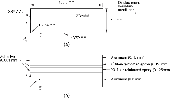
Problem description and material characteristics
Figure 1 shows the geometry of the laminate containing the blunt notch for this example. The
laminate is subjected to uniaxial tension in the longitudinal direction. The laminate is
made of three layers of aluminum and two layers of 0°/90° glass fiber-reinforced epoxy. Only
1/8 of the laminate needs to be modeled, with appropriate symmetric boundary conditions
applied as shown in Figure 2. Figure 2 also shows the through-thickness lay-up of the 1/8 model.
The material behavior of aluminum is assumed to be isotropic elastic-plastic with isotropic
hardening. The Young’s modulus is 73,800 MPa, and the Poisson’s ratio is 0.33; the isotropic
hardening data are listed in Table 1.
The material behavior of the glass fiber-reinforced epoxy layers is assumed to be
orthotropic, with stiffer response along the fiber direction and softer behavior in the
matrix. The elastic properties—longitudinal modulus, ; transverse modulus, ; shear moduli, and ; and Poisson’s ratios, and —are listed in Table 2. The subscript “L” refers to the longitudinal direction (or fiber direction), and the
subscript “T” refers to the two transverse directions orthogonal to the fiber direction.
The damage initiation and evolution behavior is also assumed to be orthotropic. Table 3 lists the ultimate values of the longitudinal failure stresses, and ; transverse failure stresses, and ; and in-plane shear failure stress, . The superscripts “t” and “c” refer to tension and compression,
respectively. The fracture energies of the fiber and matrix are assumed to be =12.5 N/mm and =1.0 N/mm, respectively.
Three material models that use the parameters listed above are considered, as follows:
The material is modeled using the damage model proposed by Linde et al. (2004). This
damage model is implemented in user subroutine UMAT and is referred to in this
discussion as the UMAT model. Details of the UMAT model are provided below.
The material is modeled using the multiscale material model in Abaqus (see Mean-Field Homogenization), and
the damage model is implemented in user subroutine USDFLD at the constituent level.
Details of the multiscale material and the damage model are provided below.
The adhesive used to bond neighboring layers is modeled using interface layers with a
thickness of t=0.001 mm. To simulate the interlaminar delamination,
these interface layers are modeled with cohesive elements. The initial elastic properties of
each interface are assumed to be isotropic with Young’s modulus E=2000
MPa and Poisson’s ratio =0.33. The failure stresses of the interface layers are assumed to be ===50 MPa; the fracture energies are ===4.0 N/mm. The subscripts “n,” “s,” and “t” refer to the normal direction
and the first and second shear directions (for further discussion of the constitutive
modeling methods used for the adhesive layers, see Defining the Constitutive Response of Cohesive Elements Using a Traction-Separation Description).
The plate is loaded with displacement boundary conditions applied at the right edge. To
simplify the postprocessing, the displacement loading is applied at a reference point and an
equation constraint is used to constrain the displacement along the loading direction
between the right edge and the reference point. Except for those files designed exclusively
to study the effect of the loading direction on the strength, the loading direction (along
the global X-direction) aligns with the fiber direction of the 0°
fiber-reinforced epoxy layer.
UMAT model for fiber-reinforced epoxy
layers
For fiber-reinforced epoxy layers, the primary model considered is based on the Hashin
damage model for unidirectional fiber-reinforced composites available in both Abaqus/Standard and Abaqus/Explicit. Alternatively, in Abaqus/Standard, the damage in the fiber-reinforced epoxy is also simulated using the model proposed by
Linde et al. (2004), which is implemented in user subroutine UMAT and is discussed below.
In the UMAT model, the damage initiation
criteria are expressed in terms of strains. Unlike the Hashin damage model in Abaqus, which uses four internal (damage) variables, the UMAT model uses two damage variables
to describe damage in the fiber and matrix without distinguishing between tension and
compression. Although the performance of the two models is expected to be similar for
monotonic loads, such as in this example problem, the results obtained might differ
considerably for more complex loads in which, for example, tension is followed by
compression. For the UMAT model, if the material is
subjected to tensile stresses that are large enough to cause partial or full damage (the
damage variable corresponding to this damage mode is greater than zero), both tensile and
compressive responses of the material are affected. However, in the case of the Hashin
damage model, only the tensile response is degraded while the material compressive response
is not affected. In many cases the latter behavior is more suitable for modeling
fiber-reinforced composites. In this section the governing equations for damage initiation
and evolution as proposed by Linde et al. (2004) are discussed, followed by a description of
the user subroutine UMAT implementation.
Damage in the fiber is initiated when the following criterion is reached:
where , , and are the components of the elasticity matrix in the undamaged state. Once
the above criterion is satisfied, the fiber damage variable, , evolves according to the equation
where is the characteristic length associated with the material point.
Similarly, damage initiation in the matrix is governed by the criterion
where , , and . The evolution law of the matrix damage variable, , is
During progressive damage the effective elasticity matrix is reduced by the two damage
variables and , as follows:
The use of the fracture energy-based damage evolution law and the introduction of the
characteristic length in the damage evolution law help to minimize the mesh sensitivity of the
numerical results, which is a common problem of constitutive models with strain softening
response. However, since the characteristic length calculation is based only on the element
geometry without taking into account the real cracking direction, some level of mesh
sensitivity remains. Therefore, elements with an aspect ratio close to one are recommended
(for a discussion of mesh sensitivity, see Concrete Damaged Plasticity).
In user subroutine UMAT the stresses are updated
according to the following equation:
The Jacobian matrix can be obtained by differentiating the above equation:
The above Jacobian matrix is not symmetric; therefore, the unsymmetric equation solution
technique is recommended if the convergence rate is slow.
To improve convergence, a technique based on viscous regularization (a generalization of
the Duvaut-Lions regularization) of the damage variables is implemented in the user
subroutine. In this technique we do not use the damage variables calculated from the
aforementioned damage evolution equations directly; instead, the damage variables are
“regularized” using the following equations:
where and are the matrix and fiber damage variables calculated according to the
damage evolution laws presented above, and are the “regularized” damage variables used in the real calculations of
the damaged elasticity matrix and the Jacobian matrix, and is the viscosity parameter controlling the rate at which the regularized
damage variables and approach the true damage variables and .
To update the “regularized” damage variables at time , the above equations are discretized in time as follows:
From the above expressions, it can be seen that
Therefore, the Jacobian matrix can be further formulated as follows:
Care must be exercised to choose an appropriate value for since a large value of viscosity might cause a noticeable delay in the
degradation of the stiffness. To estimate the effect of viscous regularization, the
approximate amount of energy associated with viscous regularization is integrated
incrementally in user subroutine UMAT by updating the variable
SCD as follows:
where is the damaged elasticity matrix calculated using the damage variables, and ; and is the damaged elasticity matrix calculated using the regularized damage
variables, and . To avoid unrealistic results due to viscous regularization, the above
calculated energy (available as output variable
ALLCD) should be small compared to the
other real energies in the system, such as the strain energy
ALLSE.
This user subroutine can be used with either three-dimensional solid elements or elements
with plane stress formulations. In the user subroutine the fiber direction is assumed to be
along the local 1 material direction. Therefore, when solid elements are used or when shell
elements are used and the fiber direction does not align with the global
X-direction, a local material orientation should be specified. The
damage variables (, , , and ) are stored as solution-dependent variables, which
can be viewed in the Visualization module of Abaqus/CAE.
Multiscale model for fiber-reinforced epoxy layers
The material of the fiber-reinforced epoxy layers is also modeled with the multiscale
material model available in Abaqus/Standard. The Mori-Tanaka homogenization method is used, and the volume fraction of the fiber is
set to 60%, which is typical for fiber-reinforced epoxy composites. Both the matrix material
and fiber material are modeled with a linear elastic material model. The elastic moduli are
calibrated to match the composite properties listed in Table 2. The matrix material is assumed to be isotropic. The Poisson's ratio is 0.41, and the
calibrated Young's modulus is 4889.0 MPa. The fiber material is modeled with transversely
isotropic linear elastic material with the calibrated properties listed in Table 4. The shape of the fiber is assumed to be cylindrical with infinite
length.
In the multiscale material model, the damage initiation criteria proposed by Meyes et al.
(2001) are used. Separate failure criteria are used for the fiber and matrix based on
different failure modes. Rather than using composite stresses to predict constituent
failure, the following transversely isotropic stress invariants are used to compute the
failure criterion for each constituent:
The stress limit values of the matrix material and fiber material are obtained from
microlevel solutions when the stress limits listed in Table 3 are reached at the composite level.
Damage in the fiber material is initiated when one of the following criteria is reached:
Fiber tension :
Fiber compression :
Damage in the matrix material is initiated when one of the following criteria is reached:
Matrix tension :
Matrix compression :
where
The parameters in the above equations are listed in Table 5. Upon damage initiation, the damage variables in the constituents are
computed using the same damage evolution model using in the Hashin model (Damage Evolution and Element Removal for Fiber-Reinforced Composites). To improve convergence, the damage variables are "regularized"
using the following equations:
The value of the "regularized" damage variable is assigned to the field variable used to
define the elastic properties of the matrix and fiber materials. The Poisson's ratios remain
unchanged while the other elastic moduli reduce by 1×10⁻⁶ when the field
variables reach 1.0.
Both damage initiation and the viscous regularization of the damage variables are
implemented in user subroutine USDFLD. The damage variables at
tension and compression failure (, , , and ) are stored as solution-dependent variables, which
can be viewed in the Visualization module of Abaqus/CAE.
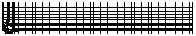
Finite element model
The finite element model uses a separate mesh for each of the respective layers shown in
Figure 2: two aluminum layers, two fiber-reinforced epoxy layers, and three adhesive layers. While
not required, a similar finite element discretization in the plane of the laminate, such as
that shown in Figure 3, can be used for all layers.
Modeling considerations for aluminum layers
Due to the interactions with the fiber-reinforced epoxy layers, the stress state within
the aluminum layers (especially surrounding the notch tip) cannot be approximated using
the plane stress assumption. To model this three-dimensional plasticity stress state
accurately, solid elements must be used for the aluminum layers. In Abaqus/Standard incompatible mode elements (C3D8I) are
used since local bending might exist in the post-failure region surrounding the notch. For
the Abaqus/Explicit analysis, reduced-integration elements
(C3D8R) are used for modeling the aluminum
layers.
Modeling considerations for glass fiber-reinforced epoxy layers
The plane stress assumption can be used safely within the fiber-reinforced epoxy layers;
therefore, either solid elements or shell elements can be adopted for these layers.
However, it is important to have an accurate representation of the through-thickness
geometry to model the interface between the adhesive and the fiber-reinforced epoxy
realistically. This is achieved most conveniently with solid elements or continuum shell
elements instead of conventional shell elements. The Hashin damage model for
unidirectional fiber-reinforced materials is available only for elements with a plane
stress formulation. Therefore, continuum shell elements are used with this model. Models
are also included in which continuum elements
(C3D8R or
C3D8) are used along with user subroutine
UMAT to model the fiber-reinforced
epoxy layers. The multiscale material model using continuum shell elements appears to give
the best results for the damage model described above. The model is also available for
plane stress elements and three-dimensional continuum solid elements.
Modeling considerations for adhesive layers
Cohesive elements (COH3D8) are used for the
interface layers. The elastic response is defined in terms of a traction-separation law
with uncoupled behavior between the normal and shear components. For convenience, a
constitutive thickness of 1.0 mm is used so that we do not need to distinguish between the
separation displacement and the nominal strain
(NE). However, since the actual
thickness is 0.001 mm, the diagonal terms in the elasticity matrix need to be scaled by
the inverse of the actual thickness as follows:
The quadratic nominal strain criterion is used for the damage initiation:
Results for each analysis are discussed in the following sections.
Abaqus/Standard results
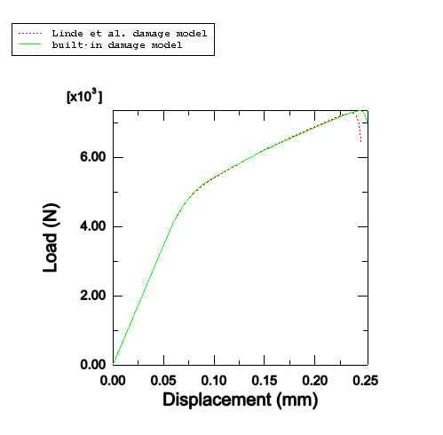
Damage to the fiber-reinforced epoxy plays a key role in the response for the loading
considered. Figure 4 shows the load-displacement curve for the 0° loading direction for the Linde and Hashin
(built-in) the damage models considered for the fiber-reinforced epoxy. The response shows
a “bilinear” shape before the sudden loss of loading capacity; that is, an initial linear
curve representing the initial elastic region, a smoothly deflecting nonlinear curve
representing the local plasticity, and a second linear curve representing the net section
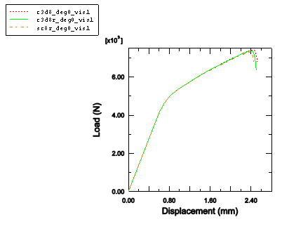
yielding. The effect of the element type was studied using the UMAT model and
C3D8R,
C3D8, and
SC8R elements; and the results are
summarized in Figure 5 and Table 7. The numerical results obtained using different element types and different damage
models are similar and show a good agreement with the experimental results of De Vries
(2001).
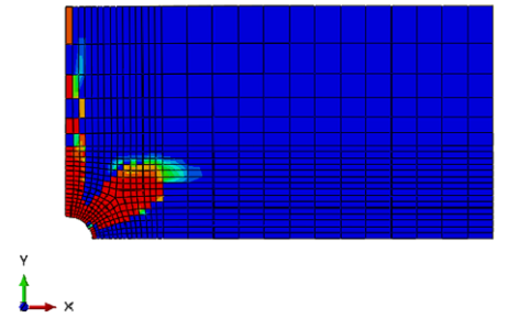
The fiber and matrix damage patterns in the 0° fiber-reinforced epoxy layer at the
failure load are shown in
Figure 6 and Figure 7, for the Hashin damage model for fiber-reinforced materials;
It can be seen that the fiber damage in the 0° fiber-reinforced epoxy layer propagates
along the ligament above the blunt notch tip (that is, orthogonal to the loading
direction).
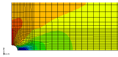
Figure 12 shows the matrix damage in the 90° layer for the damage model of Linde et al. (2004).
There is no fiber damage in the 90° fiber-reinforced epoxy layer prior to the sudden
fracture. Interlaminar damage is most severe between the 0° fiber-reinforced epoxy layer
and the aluminum layer. These observations are in agreement with the experimental results
of De Vries (2001).
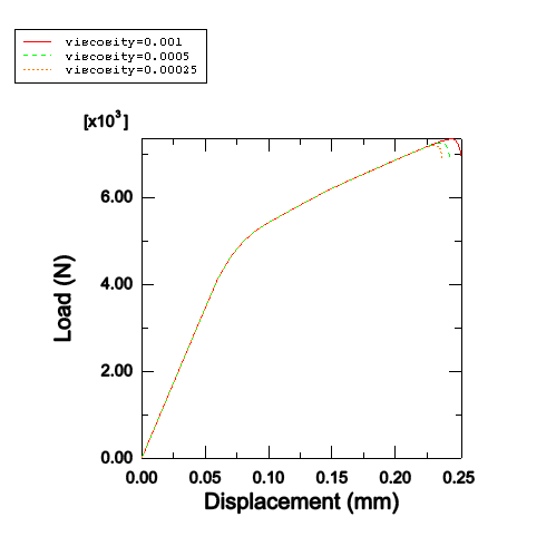
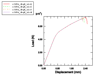
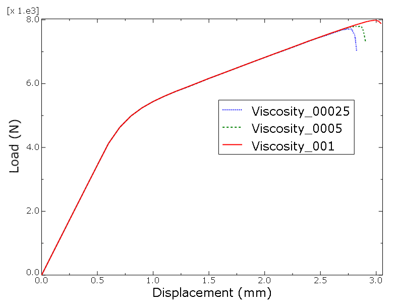
The load-displacement results for different values of the viscosity parameter, are given in
Figure 13 and Table 6, for the Hashin damage model for fiber-reinforced materials;
The smaller the viscosity, the more abrupt the failure and the smaller the failure
strength. Although a viscosity of 0.001 seems to overestimate the failure strength by a
few percent (Table 6 and Table 8), the convergence is noticeably improved. Therefore, a viscosity of 0.001 is used for
all the other studies in this example.
For the Hashin damage model for fiber-reinforced materials, only the viscosity in the
fiber direction was varied while the viscosity in the matrix direction was kept constant
at 0.005. This improved convergence and did not markedly affect the results.
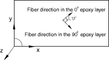
The effect of the loading direction on the blunt notch strength is studied using the
three-dimensional element, C3D8R, with the
UMAT model. Three tests are
performed in which the local material orientations in the 0°/90° fiber-reinforced epoxy
are rotated by an angle of 15°, 30°, and 45°, respectively. For example, for a loading
angle of 15° the fiber orientation in the 0° fiber-reinforced epoxy layer would be at a
15° angle with respect to the X-direction, while the fiber
orientation in the 90° fiber-reinforced epoxy layer would be at an angle of −75° with
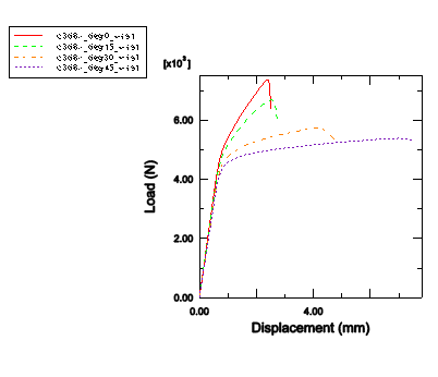
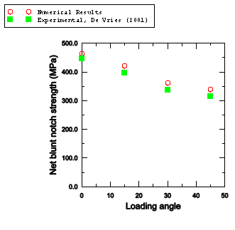
respect to the X-direction (Figure 16). As can be seen in Figure 17, strain hardening is smaller for the larger loading angles. As can be seen in Figure 18, the failure strength decreases with the increasing loading angle and reaches the
minimum at the 45° loading angle (the response for even larger loading angles is expected
to be approximately symmetric with respect to the 45° angle due to the symmetric nature of
the 0°/90° fiber-reinforced epoxy layer). As stated by De Vries (2001), this is expected
and reflects the poor shear properties of the fiber-reinforced epoxy layer.
In the above discussions the net blunt notch strength is defined as , where is the length of the ligament above the notch and t
is the total thickness of the laminate. This example demonstrates that the approach
employed in the study can be used to predict the blunt notch strength of the fiber metal
laminates.
Abaqus/Explicit results
In the Abaqus/Explicit simulation, we only consider loading along the 0° ply. The simulation is conducted
without damage stabilization, and no mass scaling is used. However, in order to reduce the
computational time, the total loading is applied in a short interval of time (0.001 s).
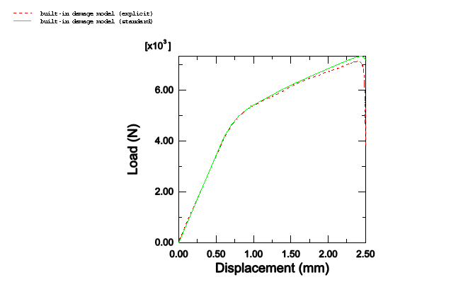
The overall load-displacement curve obtained from the explicit dynamic simulation is
compared with the Abaqus/Standard result (with viscosity of 0.001) in Figure 19. The results from the explicit dynamic simulation are presented using an antialiasing
filter to remove high frequency noise (see Filtering Output and Operating on Output in Abaqus/Explicit). The overall response compares well with the Abaqus/Standard results with some differences in the peak value of the load and in the post-peak
response. Damage stabilization is used in the Abaqus/Standard simulation to achieve convergence and is likely to change the overall response
(especially in the post-peak portion of the load-displacement curve). On the other hand,
the Abaqus/Explicit simulation does not use damage stabilization and is better able to capture the dynamic
behavior inherent in the damage and failure processes. The contour plots of various damage
variables in the 0° and 90° plies agree qualitatively with the corresponding plots
obtained from the Abaqus/Standard simulation using the Hashin damage model.
SC8R used in the fiber-reinforced
epoxy layer, a loading angle of 0°, and a viscosity of 0.001 in the fiber material
(using multiscale material model).
SC8R used in the fiber-reinforced
epoxy layer, a loading angle of 0°, and a viscosity of 0.0005 in the fiber material
(using multiscale material model).
SC8R used in the fiber-reinforced
epoxy layer, a loading angle of 0°, and a viscosity of 0.00025 in the fiber material
(using multiscale material model).
SC8R elements used in the
fiber-reinforced epoxy layer and a loading angle of 0° (using Hashin damage model).
References
De
Vries, T.J., “Blunt
and Sharp Notch Behavior of Glare
Laminates,” Ph.D dissertation, Delft
University
Press, 2001.
Hagenbeek, M., C. Van
Hengel, O. J. Bosker, and C. A. J. R. Vermeeren, “Static
Properties of Fibre Metal Laminates,” Applied
Composite
Materials, vol. 10207–222, 2003.
Linde, P., J. Pleitner, H. De
Boer, and C. Carmone, “Modelling
and Simulation of Fiber Metal Laminates,” Abaqus
Users’
Conference, 2004.
Mayes, J.S.., and A.C.. Hansen, “Multicontinuum Failure Analysis of Composite Structural Laminates,” Mechanics of Composite Materials and Structures, vol. 8, no. 4249-262, 2001.
Tables
Table 1. Isotropic hardening data for aluminum.
Yield stress (MPa)
Plastic strain (%)
300
0.000
320
0.016
340
0.047
355
0.119
375
0.449
390
1.036
410
2.130
430
3.439
450
5.133
470
8.000
484
14.710
Table 2. Orthotropic elastic properties of fiber-reinforced epoxy.
(MPa)
(MPa)
(MPa)
(MPa)
55000
9500
5500
3000
0.45
0.33
Table 3. Orthotropic damage initiation properties of fiber-reinforced epoxy.
(MPa)
(MPa)
(MPa)
(MPa)
(MPa)
2500
2000
50
150
50
Table 4. Transversely isotropic elastic properties of fiber material.
(MPa)
(MPa)
(MPa)
24490
14156
24490
0.280
0.516
Table 5. Damage initiation properties of matrix and fiber in the multiscale material.
(MPa)
(MPa)
(MPa)
(MPa)
(MPa)
(MPa)
(MPa)
(MPa)
4013
3210
45
134
3.5
10.6
33
27
Table 6. Net blunt notch strength (MPa) for different values of the viscosity parameter in
fiber direction (using Hashin damage model, viscosity in the matrix direction =0.005).
Numerical results
(SC8R, 0o loading
angle)
Experimental results(De Vries, 2001)
=0.001
=0.0005
=0.00025
462.1
456.4
453.2
446
Table 7. Net blunt notch strength (MPa) for different element types used in the
fiber-reinforced epoxy layers (using UMAT
model).
Numerical results (=0.001, 0o loading angle)
Experimental results (De Vries,
2001)
C3D8R
C3D8
SC8R
463.7
467.1
458.7
446
Table 8. Net blunt notch strength (MPa) for different values of the viscosity parameter (using
UMAT model).
Numerical results
(C3D8R, 0o
loading angle)
Experimental results(De Vries, 2001)
=0.001
=0.0004
=0.00016
=0.000064
463.7
453.8
449.2
448.2
446
Table 9. Net blunt notch strength (MPa) for different values of the viscosity parameter (using
multiscale model).
Numerical results
(SC8R, 0o loading
angle)
Experimental results(De Vries, 2001)
=0.001
=0.0005
=0.00025
454
443
439
446
Figures
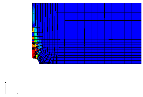
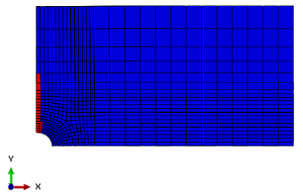
Figure 1. Plate geometry. Figure 2. (a) In-plane view of the 1/8 plate; (b) through-thickness lay-up of the 1/8
plate. Figure 3. Finite element mesh. Figure 4. Load-displacement curves for different damage models in the fiber-reinforced epoxy
layer for the 0° loading direction, =0.001. Figure 5. Load-displacement curves for different element types in the fiber-reinforced epoxy
layer for the 0° loading direction (using
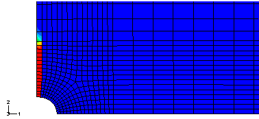
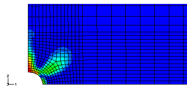
UMAT model). Figure 6. Fiber damage pattern in the 0° fiber-reinforced epoxy layer for the 0° loading
direction (using the Hashin damage model,
DAMAGEFT contour plot). Figure 7. Matrix damage pattern in the 0° fiber-reinforced epoxy layer for the 0° loading
direction (using the Hashin damage model,
DAMAGEMT contour plot). Figure 8. Fiber damage pattern in the 0° fiber-reinforced epoxy layer for the 0° loading
direction (using UMAT model,
SDV3 contour plot). Figure 9. Matrix damage pattern in the 0° fiber-reinforced epoxy layer for the 0° loading
direction (using UMAT model,
SDV4 contour plot). Figure 10. Fiber damage pattern in the 0° fiber-reinforced epoxy layer for the 0° loading
direction (using multiscale material model,
FV1_fiber contour plot). Figure 11. Matrix damage pattern in the 0° fiber-reinforced epoxy layer for the 0° loading
direction (using multiscale material model,
FV1_matrix contour plot). Figure 12. Matrix damage pattern in the 90° fiber-reinforced epoxy layer for the 0° loading
direction (using UMAT model,
SDV4 contour plot). Figure 13. Load-displacement curves for different values of the viscosity parameter for the 0°
loading direction (using the Hashin damage model). Figure 14. Load-displacement curves for different values of the viscosity parameter for the 0°
loading direction (using UMAT). Figure 15. Load-displacement curves for different values of the viscosity parameter for the 0°
loading direction (using multiscale material model). Figure 16. Local material orientations in the fiber-reinforced epoxy layers for the 15° loading
direction. Figure 17. Load-displacement curves for different loading directions (using
UMAT model). Figure 18. Calculated blunt notch strength for different loading angles in comparison with the
experimental results (using UMAT
model). Figure 19. Load-displacement curves for the 0° loading direction: Abaqus/Explicit versus Abaqus/Standard.