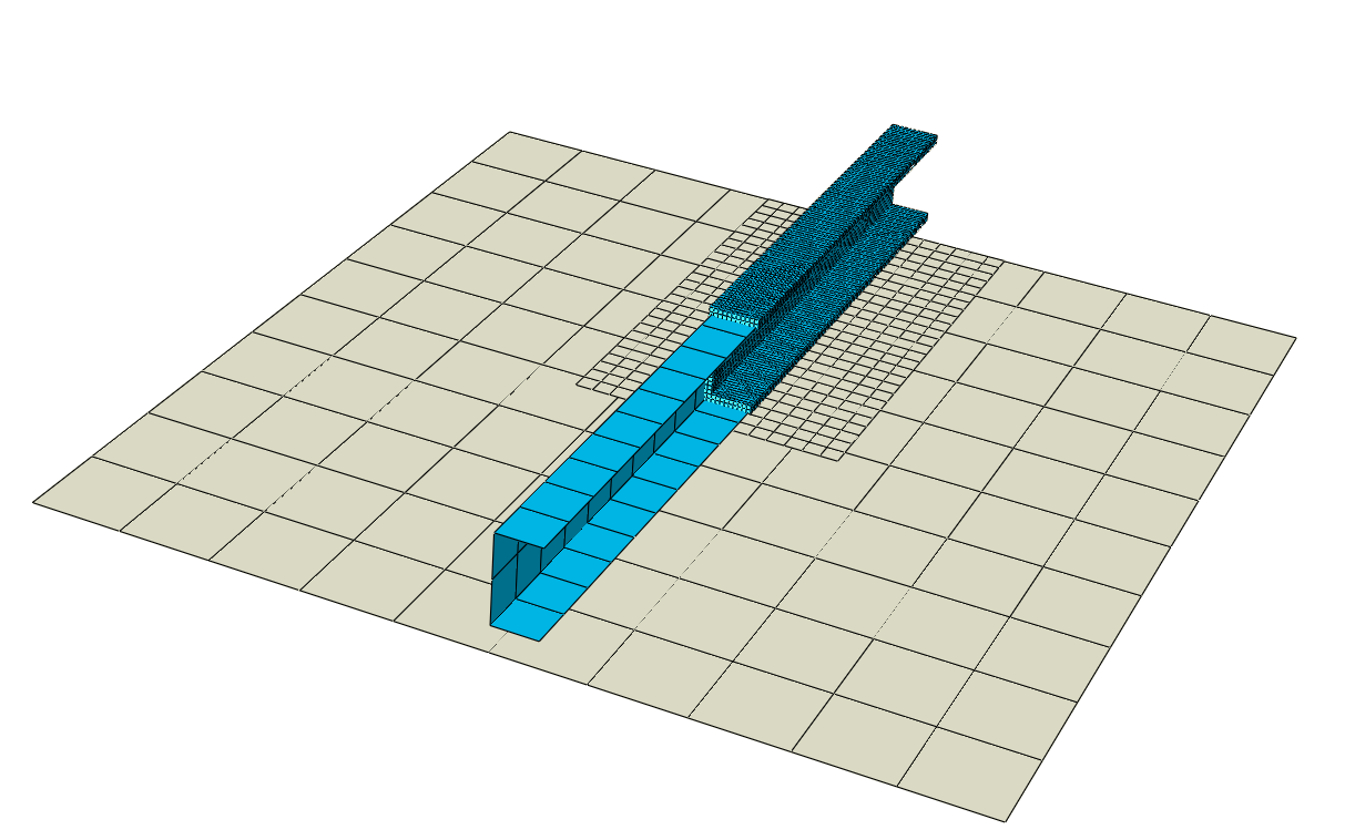
General submodeling imposes the displacements, rotations, temperatures, or
pore pressure obtained from the beam, solid, or shell elements in the global model onto
a surface defined in the submodel.
The surface in the submodel is meshed
with either beam, solid, or shell elements.
General submodeling enables a strategy to use beam, solid, and shell elements in a
global model to obtain an approximate solution efficiently followed by a submodel
with beam, solid, or shell elements to study a region in more detail. Results from
the global model impose conditions on cut surfaces of the submodel.
General Submodeling
Element Types Supported
General submodeling uses beam elements, solid elements, or shell elements in the
submodel.
Procedures Supported
Both the global model and the submodel can have nonlinear response and can be
analyzed for any sequence of analysis procedures. These procedures do not have
to be the same for both models. For example, the linear dynamic response of the
global model can be used to drive the static, nonlinear response of the submodel
on the grounds that the submodel is too small for dynamic effects to be
significant in that local region. You cannot use general submodeling in Abaqus/Explicit analyses.
Your submodel cannot refer to a global model step that includes multiple load
cases (see Multiple Linear Load Case Analysis). You must perform the
global analysis with a single load definition for the step that will drive the
submodel.
Invoking General Submodeling
Creating and executing a submodel in the context of general submodeling involves the
following:
Specifying the named element-based surfaces that will be associated with
submodel cuts as model data.
Using the named surfaces to define submodel cuts as part of the model data .
Specifying data that are common to all submodel cuts, such as the associated
step and increment of the global model, as part of the submodel conditions
definition for a step.
Specifying the name of the associated global model with the
globalmodel parameter on the Abaqus command line.
General submodeling imposes boundary conditions on primary degrees of freedom of the
nodes on the cut surface either directly or by defining a distributed coupling
element on the nodes of the cut surface. The following primary degrees of freedom
can be imposed: displacement, rotation, temperature, pore pressure, and acoustic
pressure. When the distributed coupling is defined, Abaqus/Standard imposes the boundary conditions on the reference node.
When you define the submodel cut surface on a beam cross-section or shell thickness,
Abaqus/Standard internally generates a distributing coupling with the nodes on the cut surfaces
acting as cloud nodes. Figure 1 shows superimposed global and local models for
beam-to-solid and beam-to-shell submodeling examples. These distributing couplings
are represented with lines from the reference node to each of the cloud nodes at the
four submodel cuts in Figure 1. Reference nodes for these distributing couplings are
located at the intersection of the plane of the cut surface and the beam element
reference line in the global model. Abaqus/Standard obtains the values of the imposed degrees of freedom at the reference node in the
submodel by interpolation from the global model solution for the beam element at the
location of the intersection. The distributing coupling causes the average
displacement and rotation of the cut surface to match that of the reference node,
without imposing rigidity. For example, the distributing coupling does not prevent
warping of the cut surface during the submodel simulation. Figure 1. Superimposed global and local models for beam-to-solid (left) and
beam-to-shell (right) submodeling.
Figure 2 shows the superimposed global
model and submodel for a case involving shell-to-shell and shell-to-solid
submodeling together at different submodel cuts of one submodel. The coupling method
used to impose conditions from the global model on a submodel for shell-to-shell
submodeling involves interpolation from the global model results. Figure 3 shows the coupling method for
shell-to-solid submodeling using internally generated distributing couplings with
cloud nodes on the cut surface of the submodel. The automated algorithm determines
the number of reference nodes and their positions on the submodel interface.
Displacements and rotations at reference nodes of the distributing couplings are
interpolated from shell nodes of the global model. Each of the driven solid nodes
belongs to a single distributing coupling.
Figure 2. Superimposed global and submodel for a global model with shell elements and a
submodel with a combination of shell and solid elements. Figure 3. Representation of automatically generated couplings to enforce shell-to-solid
submodeling conditions on a solid surface submodel cut.
When you define the cut surface on the edges of shell elements and you impose the
boundary conditions from shell elements in the global model using interpolation, you
do not need distributing coupling elements.
Modifying the Imposed Conditions
By default, Abaqus/Standard imposes all primary degrees of freedoms that are common to both the global
model and submodel on all cut surfaces. You can specify the degrees of freedoms
to be imposed and the degrees of freedom to be excluded for each of the cut
surfaces.
Input File Usage
Use following data lines:
SUBMODEL CONDITIONScut surface name, First dof, Last dof, Por N, First dof, Last dof, P, or Ncut surface name, First dof, Last dof, Por N
...
If you omit the name of the cut surface, the specification refers to all
cut surfaces.
Enter the letter P to impose the primary
degrees of freedom and the letter N to
exclude the primary degrees of freedom.
Use a separate data line for each cut surface to modify the imposed
conditions. The last specification takes precedence over any earlier
specification.
Consistent Configuration and Orientation
Accurate submodel behavior for submodeling from a beam element in the global model
requires consistency of the beam cross-section configuration in the global model and
submodel. Initial nodal positions of the submodel must account for:
Beam section offset in the global model.
The orientation of principal beam axes in the global model.
Beam section dimensions and thicknesses.
Referring to the Step and Increment of the Global Model
Step histories often match between a submodel and the corresponding global model. In
these cases and some other cases with differences in step histories (as explained in
Figure 4 and Figure 5), the following default conventions for step
synchronization (that is, associating the steps of a submodel with a global model)
are appropriate:
The ith general step of a submodel is driven by the
ith general step of the associated global
model.
The jth perturbation step associated with a base
state determined by the ith general step of a
submodel is driven by the jth perturbation step
determined by the ith general step of the associated
global model.
In the example shown in Figure 4, the
global model has an extra perturbation step after the second general step compared
to the submodel. In this case, by default, the extra perturbation step is not used
to drive the submodel conditions. Default step synchronization is reasonable for
this example. However, if, for example, you intended to have Step 3 of the submodel
driven by Step 4 of the global model, you could override the default.Figure 4. Example of default time synchronization referencing from submodel steps
to global model steps that drive submodel conditions.
Figure 5 shows a similar example, but
with an extra perturbation step in the submodel relative to the global model. In
this case Abaqus issues an error message if you are using the default time synchronization because
the global model only has one perturbation step after the second global step. For
example, you could specify that Step 4 of the submodel (which is a perturbation
step) should be driven by perturbation results from Step 5 of the global model, even
though Step 5 of the global model uses a different base state. Such an association
might be questionable, but it is not disallowed.
Figure 5. Example with default time synchronization unable to determine the default
driving global step for one step of the submodel.
Figure 6 shows two examples of
nondefault time synchronization references for submodeling. Both models consider the
same four general steps, and default time synchronization reasonably applies to
these general steps. Step 3 of the submodel is a perturbation step that the user has
explicitly specified should be driven by incremental changes determined in the first
increment of Step 3 of the global model.
Figure 6. Example with default time synchronization used for four general steps of a
submodel and nondefault synchronization specified for two of three perturbation
steps of a submodel.
Amplitude Scaling Between the Global Model and Submodel
Amplitude scaling enables you to scale the results of the global model that are used
to drive conditions at submodel cuts. For example, an amplitude scale factor of 2.0
doubles the driven conditions at a submodel cut. The default scale factor is
1.0.
Time Scaling Between the Global Model and Submodel
Time periods of corresponding steps of a submodel and global model might differ. Time
scaling occurs by default, such that the variations of driving conditions are based
on fractional step completion of the global step and corresponding submodel
step.
You can optionally deactivate time scaling. For example, if a global step has a
period of 1.0 seconds and the corresponding submodel step has a period of 2.0
seconds, the time histories of conditions driving the submodel will match for the
first second but will remain constant for the last half of the submodel step. This
approach might be appropriate for a global model step with purely static behavior
(which does not involve a physical time period) and a corresponding submodel step
with transient static response involving time-dependent material behavior (creep,
swelling, and viscoelasticity).
Controls Associated with Identifying the Global Element Associated with a Cut
Surface
A search algorithm identifies global elements associated with each local cut surface.
The default search algorithm is usually sufficient. Optionally, you can specify a
global element set as input to this algorithm to limit which global elements are
considered as candidates. If a cut surface of the local model corresponds to the
location of a node shared by multiple beam elements in the global model, specifying
one of these elements in a global element set removes uncertainty about which global
element is chosen to drive the submodel conditions at that cut. Similarly, you can
define tolerances to include or exclude entities that lie outside the boundaries of
the submodel. You can specify the tolerances either as a percentage of the average
element size or as absolute values.
Input File Usage
Use following option.
SUBMODEL CUT, ABSOLUTE EXTERIOR TOLERANCE=value, EXTERIOR TOLERANCE=value, GLOBAL ELSET=element_set_name
Using Multiple Linear Load Cases in a Submodel
Multiple linear load case functionality (see Multiple Linear Load Case Analysis) can be used in the context of general submodeling, which reduces memory and
execution time compared to defining separate perturbation steps. Load cases can
exist both in the global model analysis and in the submodel analysis. If the global
step being referenced in a submodel analysis has multiple linear load cases, you
must specify the name of the load case in the global model.
There are two methods that you can use for a submodel to refer to linear load cases
of a global model, as follows:
The first method allows multiple linear load cases to be considered in a
single submodel step. In this case, you must assign names to the linear load
cases in the context of the submodel step.
This method is the most
efficient way to consider multiple load cases associated with a common
base state.
The second method allows only one linear load case to be referenced per
submodel step. This method does not require you to assign a name to the
linear load case in the context of the submodel step.
However, this method
increases simulation time compared to the first method because some
computations are repeated in each step.
The usage example below refers to the same two linear load cases of the global
model as the previous submodel usage example. However, this example uses the
second method, which increases simulation time
compared.
Submodel analysis is identical to any other analysis. You can request all output
variables that are appropriate to the procedure.
Limitations
General submodeling is subject to the following limitations:
Elements for forced convection/diffusion are not supported.
Elements with coupled thermal-electrical fields are not supported.
Piezoelectric elements are not supported.
Electromagnetic elements are not supported.
Coupled thermal-electrochemical, coupled thermal-electrochemical-structural,
and coupled thermal-electrochemical-structural-pore pressure elements are
not supported.
Gasket elements, cylindrical elements, and surface elements are not
supported.
Special-purpose elements such as cohesive elements, fluid pipe elements,
drag chain elements, Eulerian elements, pipe-soil elements, spring elements,
and acoustic-interface elements are not supported.