Abaqus provides a set of elements for modeling a fluid medium undergoing small pressure variations
and interface conditions to couple these acoustic elements to a structural model. These
elements are provided to model a variety of phenomena involving dynamic interactions between
fluid and solid media.
Steady-state harmonic (linear) response analysis can be performed for a coupled
acoustic-structural system, such as the study of the noise level in a vehicle. The
steady-state procedure is based on direct solution of the coupled complex harmonic equations,
as described in Direct steady-state dynamic analysis; on a modal-based procedure, as
described in Steady-state linear dynamic analysis; or on a subspace-based procedure, as
described in Subspace-based steady-state dynamic analysis. Mode-based linear transient dynamic
analysis is also available, as described in Modal dynamic analysis.
The acoustic fluid elements can also be used with nonlinear response analysis (implicit or
explicit direct integration) procedures: whether such results are useful depends on the
applicability of the small pressure change assumption in the fluid. Often in coupled
fluid-solid problems the fluid forces in this linear regime are high enough that nonlinear
response of the structure needs to be considered. For example, a ship subjected to underwater
incident wave loads due to an explosion may experience plastic deformation or large motions of
internal machinery may occur.
The acoustic medium in Abaqus may have velocity-dependent dissipation, caused by fluid viscosity or by flow within a
resistive porous matrix material. In addition, rather general boundary conditions are provided
for the acoustic medium, including impedance, or “reactive,” boundaries.
The possible conditions at the surface of the acoustic medium are:
Prescribed pressure (degree of freedom 8) at the boundary nodes. (Boundary conditions can
be used to specify pressure at any node in the model.)
Prescribed inward normal derivative of pressure per unit density of the acoustic medium
through the use of a concentrated load on degree of freedom 8 of a boundary node. If the
applied load has zero magnitude (that is, if no concentrated load or other boundary
condition is present), the inward normal derivative of pressure (and normal fluid particle
acceleration) is zero, which means that the default boundary condition of the acoustic
medium is a rigid, fixed wall (Neumann condition).
Acoustic-structural coupling defined either by using surface-based coupling procedures
(see Surface-based acoustic-structural medium interaction) or by placing
ASI coupling elements on the interface
between the acoustic medium and a structure.
An impedance condition, representing an absorbing boundary between the acoustic medium
and a rigid wall or a vibrating structure or representing radiation to an infinite
exterior.
An incident wave loading, representing the inward normal derivative of pressure per unit
density of the acoustic medium resulting from the arrival of a specified wave. The
formulation of this loading case is discussed in Loading due to an incident dilatational wave field.
It is applicable to problems involving blast loads and to acoustic scattering problems.
The flow resistance and the properties of the absorbing boundaries may be functions of
frequency in steady-state response analysis but are assumed to be constant in the direct
integration procedure. This section defines the formulation used in these elements.
Acoustic equations
The equilibrium equation for small motions of a compressible, adiabatic fluid with
velocity-dependent momentum losses is taken to be
where p is the excess pressure in the fluid (the pressure in excess of
any static pressure); is the spatial position of the fluid particle; is the fluid particle velocity; is the fluid particle acceleration; is the density of the fluid; is the “volumetric drag” (force per unit volume per velocity); and are i independent field variables such as
temperature, humidity of air, or salinity of water on which and may depend (see Acoustic Medium). The d'Alembert
term has been written without convection on the assumption that there is no steady flow of
the fluid. This is usually considered sufficiently accurate for steady fluid velocities up
to Mach 0.1.
The constitutive behavior of the fluid is assumed to be inviscid, linear, and compressible,
so
where is the bulk modulus of the fluid.
For an acoustic medium capable of undergoing cavitation, the absolute pressure (sum of the
static pressure and the excess dynamic pressure) cannot drop below the specified cavitation
limit. When the absolute pressure drops to this limit value, the fluid is assumed to undergo
free expansion without a corresponding drop in the dynamic pressure. The pressure would
rebuild in the acoustic medium once the free expansion that took place during the cavitation
is reversed sufficiently to reduce the volumetric strain to the level at the cavitation
limit. The constitutive behavior for an acoustic medium capable of undergoing cavitation can
be stated as
where a pseudopressure , a measure of the volumetric strain, is defined as
where is the fluid cavitation limit and is the initial acoustic static pressure. A total wave formulation is used
for a nonlinear acoustic medium undergoing cavitation. This formulation is very similar to
the scattered wave formulation presented below except that the pseudopressure, defined as
the product of the bulk modulus and the compressive volumetric strain, plays the role of the
material state variable instead of the acoustic excess pressure. The acoustic excess
pressure is readily available from this pseudopressure subject to the cavitation condition.
Physical boundary conditions in acoustic analysis
Acoustic fields are strongly dependent on the conditions at the boundary of the acoustic
medium. The boundary of a region of acoustic medium that obeys Equation 1 and Equation 2 can be divided into subregions S on which the following conditions
are imposed:
,
where the value of the acoustic pressure p is prescribed.
,
where we prescribe the normal derivative of the acoustic medium. This condition also
prescribes the motion of the fluid particles and can be used to model acoustic
sources, rigid walls (baffles), incident wave fields, and symmetry planes.
,
the “reactive” acoustic boundary, where there is a prescribed linear relationship
between the fluid acoustic pressure and its normal derivative. Quite a few physical
effects can be modeled in this manner: in particular, the effect of thin layers of
material, whose own motions are unimportant, placed between acoustic media and rigid
baffles. An example is the carpet glued to the floor of a room or car interior that
absorbs and reflects acoustic waves. This thin layer of material provides a “reactive
surface,” or impedance boundary condition, to the acoustic medium. This type of
boundary condition is also referred to as an imposed impedance, admittance, or a
“Dirichlet to Neumann map.”
,
the “radiating” acoustic boundary. Often, acoustic media extend sufficiently far from
the region of interest that they can be modeled as infinite in extent. In such cases
it is convenient to truncate the computational region and apply a boundary condition
to simulate waves passing exclusively outward from the computational region.
,
where the motion of an acoustic medium is directly coupled to the motion of a solid.
On such an acoustic-structural boundary the acoustic and structural media have the
same displacement normal to the boundary, but the tangential motions are uncoupled.
,
an acoustic-structural boundary, where the displacements are linearly coupled but not
necessarily identically equal due to the presence of a compliant or reactive
intervening layer. This layer induces an impedance condition between the relative
normal velocity between acoustic fluid and solid structure and the acoustic pressure.
It is analogous to a spring and dashpot interposed between the fluid and solid
particles. As implemented in Abaqus, an impedance boundary condition surface does not model any mass associated with
the reactive lining; if such a mass exists, it should be incorporated into the
boundary of the structure.
,
a boundary between acoustic fluids of possibly differing material properties. On such
an interface, displacement continuity requires that the normal forces per unit mass on
the fluid particles be equal. This quantity is the natural boundary traction in Abaqus, so this condition is enforced automatically during element assembly. This is also
true in one-dimensional analysis (that is, piping or ducts), where the relevant
acoustic properties include the cross-sectional areas of the elements. Consequently,
fluid-fluid boundaries do not require special treatment in Abaqus.
Formulation for direct integration transient dynamics
In Abaqus the finite element formulations are slightly different in direct integration transient
and steady-state or modal analyses, primarily with regard to the treatment of the volumetric
drag loss parameter and spatial variations of the constitutive parameters. To derive a
symmetric system of ordinary differential equations for implicit integration, some
approximations are made in the transient case that are not needed in steady state. For
linear transient dynamic analysis, the modal procedure can be used and is much more
efficient.
To derive the partial differential equation used in direct integration transient analysis,
we divide Equation 1 by , take its gradient with respect to , neglect the gradient of , and combine the result with the time derivatives of Equation 2 to obtain the equation of motion for the fluid in terms of the fluid pressure:
The assumption that the gradient of is small is violated where there are discontinuities in the quantity (for example, on the boundary between two elements that have a different value).
Variational statement
An equivalent weak form for the equation of motion, Equation 3, is obtained by introducing an arbitrary variational field, , and integrating over the fluid:
Green's theorem allows this to be rewritten as
Assuming that p is prescribed on , the equilibrium equation, Equation 1, is used on the remainder of the boundary to relate the pressure gradient to the motion
of the boundary:
Using this equation, the term is eliminated from Equation 4 to produce
where, for convenience, the boundary “traction” term
has been introduced.
Except for the imposed pressure on , all the other boundary conditions described above can be formulated in
terms of . This term has dimensions of acceleration; in the absence of volumetric
drag, this boundary traction is equal to the inward acceleration of the particles of the
acoustic medium:
When volumetric drag is present, the boundary traction is the normal derivative of the
pressure field, divided by the true mass density: a force per unit mass of fluid.
Consequently, when volumetric drag exists in a transient acoustic model, a unit of yields a lower local volumetric acceleration, due to drag losses.
In direct integration transient dynamics, we enforce the acoustic boundary conditions as
follows:
On ,
p is prescribed and .
On ,
where we prescribe the normal derivative of the acoustic pressure per unit density:
In the absence of volumetric drag in the medium, this enforces a value of fluid
particle acceleration, . An imposed can be used to model the oscillations of a rigid plate or body
exciting a fluid, for example. A special case of this boundary condition is , which represents a rigid immobile boundary. As mentioned above,
if the medium has nonzero volumetric drag, a unit of imposed at the boundary will result in a relatively lower imposed
particle acceleration. Incident wave fields on a boundary of a fluid are modeled
with a that varies in space and time, corresponding to the effect of the
arrival of the wave on the boundary. See Loading due to an incident dilatational wave field.
On ,
the reactive boundary between the acoustic medium and a rigid baffle, we apply a
condition that relates the velocity of the acoustic medium to the pressure and rate
of change of pressure:
where and are user-prescribed parameters at the boundary. This equation is
in the form of an admittance relation; the impedance expression is simply the
inverse. The layer of material, in admittance form, acts as a spring and dashpot in
series distributed between the acoustic medium and the rigid wall. The spring and
dashpot parameters are and , respectively; they are per unit area of the acoustic boundary.
Using this definition for the fluid velocity, the boundary tractions in the
variational statement become
On ,
the radiating boundary, we apply the radiation boundary condition by specifying the
corresponding impedance:
the acoustic-structural interface, we apply the acoustic-structural interface
condition by equating displacement of the fluid and solid, which enforces the
condition
where is the displacement of the structure. In the presence of
volumetric drag, it follows that the acoustic boundary traction coupling fluid to
solid is
In Abaqus/Standard the formulation of the transient coupled problem would be made nonsymmetric by
the presence of the term . In the great majority of practical applications, the acoustic
tractions associated with volumetric drag are small compared to those associated
with fluid inertia,
so this term is ignored in transient analysis:
On ,
the mixed impedance boundary and acoustic-structural boundary, we apply a condition
that relates the relative outward velocity between the acoustic medium and the
structure to the pressure and rate of change of pressure:
This relative normal velocity represents a rate of compression (or extension) of
the intervening layer. Applying this equation to the definition of , we obtain for the transient case
This expression for is the sum of its definitions for and . In the steady-state case the effect of volumetric drag on the
structural displacement term in the acoustic traction is included:
These definitions for the boundary term, , are introduced into Equation 6 to give the final variational statement for the acoustic medium (this is the equivalent
of the virtual work statement for the structure):
The structural behavior is defined by the virtual work equation,
where is the stress at a point in the structure, p is the
pressure acting on the fluid-structural interface, is the outward normal to the structure, is the density of the material, is the mass proportional damping factor (part of the Rayleigh damping
assumption for the structure), is the acceleration of a point in the structure, is the surface traction applied to the structure, is a variational displacement field, and is the strain variation that is compatible with . For simplicity in this equation all other loading terms except the
fluid pressure and surface traction have been neglected: they are imposed in the usual way.
The discretized finite element equations
Equation 14 and Equation 15 define the variational problem for the coupled fields and p. The problem is discretized by introducing
interpolation functions: in the fluid , up to the number of pressure nodes and in the structure , up to the number of displacement degrees of freedom. In these and the
following equations, we assume summation over the superscripts that refer to the degrees
of freedom of the discretized model. We also use the superscripts , to refer to pressure degrees of freedom in the fluid and , to refer to displacement degrees of freedom in the structure. We use a
Galerkin method for the structural system; the variational field has the same form as the
displacement: . For the fluid we use but with the subsequent Petrov-Galerkin substitution
The new function makes the single variational equation obtained from summing Equation 14 and Equation 15 dimensionally consistent:
where, for simplicity, we have introduced the following definitions:
where is the strain interpolator. This equation defines the discretized model.
We see that the volumetric drag-related terms are “mass-like”; that is, proportional to
the fluid element mass matrix.
The term is the nodal right-hand-side term for the acoustical degree of freedom , or the applied “force” on this degree of freedom. This term is obtained
by integration of the normal derivative of pressure per unit density of the acoustic
medium over the surface area tributary to a boundary node.
In the case of coupled systems where the forces on the structure due to the fluid— are very small compared to the rest of the structural forces—the system
can be solved in a “sequentially coupled” manner. The structural equations can be solved
with the term omitted; that is, in an analysis without fluid coupling.
Subsequently, the fluid equations can be solved, with imposed as a boundary condition. This two-step analysis is less
expensive and advantageous for systems such as metal structures in air.
Time integration
The equations are integrated through time using the standard implicit (Abaqus/Standard) and explicit (Abaqus/Explicit) dynamic integration options. From the implicit integration operator we obtain
relations between the variations of the solution variables (here represented by ) and their time derivatives:
The equations of evolution of the degrees of freedom can be written for the implicit case
as
The linearization of this equation is
where and are the corrections to the solution obtained from the Newton iteration, is the structural stiffness matrix, and is the structural damping matrix. These equations are symmetric if the
constituent stiffness, damping, and mass matrices are symmetric.
For explicit integration the fluid mass matrix is diagonalized in a manner similar to the
treatment of structural mass. The explicit central difference procedure described in Explicit dynamic analysis is applied to the coupled system of equations.
Summary of additional approximations of the direct integration transient
formulation
As mentioned above, derivation of symmetric ordinary differential equations in the
presence of volumetric drag requires some approximations in addition to those inherent in
any finite element method. First, the spatial gradients of the ratio of volumetric drag to
mass density in the fluid are neglected. This may be important in lossy, inhomogeneous
acoustic media. Second, to maintain symmetry, the effect of volumetric drag on the
fluid-solid boundary terms is neglected. Finally, the effect of volumetric drag on the
radiation boundary conditions is approximate. If any of these effects is expected to be
significant in an analysis, the user should realize that the results obtained are
approximate.
Formulation for steady-state response using nodal degrees of freedom
The direct-solution steady-state dynamic analysis procedure is to be preferred over the
transient formulation if volumetric drag is significant. This formulation uses the nodal
degrees of freedom in the solid and acoustic regions directly to form a large linear system
of equations defining the coupled structural-acoustic mechanics at a single frequency. If
volumetric drag effects are not significant, the mode-based procedures (see below) are
preferred because of their efficiency.
All model degrees of freedom and loads are assumed to be varying harmonically at an angular
frequency , so we can write
where is the constant complex amplitude of the variable . Thus,
We begin with the equilibrium equation
and use the harmonic time-derivative relations to obtain
We define the complex density, , as
and, thus, write
The equilibrium equation is now in a form where the density is complex and the acoustic
medium velocity does not enter. We divide this equation by and combine it with the second time derivative of the constitutive law,
Equation 2, to obtain
We have not used the assumption that the spatial gradient of is small, as was done in the transient dynamics formulation.
Variational statement
The development of the variational statement parallels that for the case of transient
dynamics, as though the volumetric drag were absent and the density complex. The
variational statement is
Integrating by parts, we have
In steady state the boundary traction is defined as
This expression is not the Fourier transform of the boundary traction defined above for
the transient case. The steady-state definition is based on the complex density and
includes the volumetric drag effect in such a way that it is always equal to the
acceleration of the fluid particles. The application of boundary conditions may be
slightly different for some cases in steady state due to this definition of the traction.
On ,
is prescribed, analogous to transient analysis.
On ,
we prescribe
The condition is enforced, even in the presence of volumetric drag.
On ,
the reactive boundary between the acoustic medium and a rigid baffle, we apply
On ,
the radiating boundary, we apply the radiation boundary condition impedance in the
same form as for the reactive boundary but with the parameters as defined in Equation 42 and Equation 43.
On ,
the acoustic-structural interface, we equate the displacement of the fluid and
solid as in the transient case. However, the acoustic boundary traction coupling
fluid to solid,
can be applied without affecting the symmetry of the overall formulation.
Consequently, the acoustic tractions in the steady-state case make no assumptions
about volumetric drag.
On ,
the mixed impedance boundary and acoustic-structural boundary, the condition
results in the definition
In this case the effect of volumetric drag is included without approximation.
The final variational statement becomes
This equation is formally identical to Equation 4, except for the pressure “stiffness” term, the radiation boundary conditions, and the
imposed boundary traction term. Because the volumetric drag effect is contained in the
complex density, the acoustic-structural boundary term in this formulation does not have
the limitation that the volumetric drag must be small compared to other effects in the
acoustic medium. In addition, in this formulation the applied flux on an acoustic boundary
represents the inward acceleration of the acoustic medium, whether or not the volumetric
drag is large. Finally, the radiation boundary conditions do not make any approximations
with regard to the volumetric drag parameter.
The above equation uses the complex density, . We manipulate it into a form that has real coefficients and an
additional time derivative through the relations
to obtain
The discretized finite element equations
Applying Galerkin's principle, the finite element equations are derived as before. We
arrive again at Equation 17 with the same matrices except for the damping and stiffness matrices of the acoustic
elements and the surfaces that have imposed impedance conditions, which now appear as
The matrix modeling loss to volumetric drag is proportional to the fluid stiffness matrix
in this formulation.
For steady-state harmonic response we assume that the structure undergoes small harmonic
vibrations, identified by the prefix , about a deformed, stressed base state, which is identified by the
subscript . Hence, the total stress can be written in the form
where
is the stress in the base state;
is the elasticity matrix for the material;
is the stiffness proportional damping factor chosen for the material (to
give the stiffness proportional contribution to the Rayleigh damping, thus introducing
the viscous part of the material behavior); and
from the discretization assumption.
To solve the steady-state problem, we assume that the governing equations are satisfied
in the base state, and we linearize these equations in terms of the harmonic oscillations.
For the internal force vector this yields
and Equation 17 can be rewritten, using the time-harmonic relations, as with
(this stiffness includes the initial stress matrix, so “stress stiffening” and
“load stiffness” effects associated with the base state stress and loads are included) and
We have also added the “global” parts of the “structural damping” terms
and
to the equation. These damping terms model finite energy loss in the
low-frequency limit in steady-state dynamics—see Direct steady-state dynamic analysis
and Subspace-based steady-state dynamic analysis. It should be noted that the acoustic
“structural damping” operator inherits the frequency dependence of the acoustic stiffness
matrix caused by volumetric drag.
We assume that the loads and (because of linearity) the response are harmonic; hence, we
can write
and
where
, , , and
are the real and imaginary parts of the amplitudes of the
response;
and
are the real and imaginary parts of the amplitude of the force applied to
the structure;
and
are the real and imaginary parts of the amplitude of the acoustic traction
(dimensions of volumetric acceleration) applied to the fluid; and
is the circular frequency.
We substitute these equations into Equation 23 and use the time-harmonic form of Equation 16, , which yields the coupled complex linear equation system where
and
If is symmetric, Equation 24 is symmetric. The system may be quite large, because the real and imaginary parts of
the structural degrees of freedom and of the pressure in the fluid all appear in the
system. This set of equations is solved for each frequency requested in the
direct-solution steady-state dynamics procedure. If damping is absent, the user can
specify that only the real matrix equation should be factored in the analysis. Nonzero
volumetric drag values () for the acoustic medium and nonzero values for the impedances represent damping. As mentioned above for the
transient case, the coupled system can be split into an uncoupled structural analysis and
an acoustic analysis driven by the structural response, provided the fluid forces on the
structure are small.
Formulation for eigenvalue extraction and mode-based procedures
From the discretized equation, Equation 17, we can write the frequency domain problem as
where is a natural (as opposed to forced response) frequency. The indices have
been suppressed for brevity. This system is due to Zienkiewicz and Newton (1969) and is used in Abaqus as the starting point for mode-based procedures. Suppressing any damping terms, forcing,
and any terms associated with a reactive surface,
Interpreted as a linear eigenvalue problem (where is the eigenvalue), this equation cannot be solved directly in Abaqus due to the unsymmetric stiffness and mass matrices. However, it can be shown that these
equations do yield real-valued natural frequencies and modes, suggesting that they can be
rewritten in symmetric forms.
Application of the modes of Equation 25 to form a reduced system (see below) must be done with some caution, since this
unsymmetric system has distinct left and right eigenvector sets. In particular, the
“singular modes” associated with zero frequency are of interest because they describe the
low-frequency limiting behavior of the system (or the “rigid-body motion” in a kinematic
sense) and are, therefore, essential for the construction of an accurate projected frequency
domain operator. The right singular modes of the coupled system are
In other words, there is a “structural” singular right mode associated with the kernel of and an “acoustic” singular right mode associated with the kernel of . The left singular modes are solutions to
and are
The right acoustic and left structural singular modes are coupled, with
nontrivial fields on the structural and acoustic domains. These coupled singular modes are a
consequence of the stiffness term in Equation 25, and they must be computed if this system is to be projected.
An alternative frequency domain formulation, due to Everstine
(1981), involves the substitution and results in a formally symmetric system:
The corresponding coupled eigenproblem is quadratic, but the singular mode
structure of this system is much simpler—the left and right pairs are identical due to
symmetry, and the singular modes are uncoupled due to the diagonal structure of the
stiffness matrix. The modes are simply
Lanczos formulation
Introducing an auxiliary variable, , augmenting the system of equations with , and manipulating the equations yields
This augmented system of equations is due to Ohayon and is used only for Lanczos
eigenvalue extraction. The auxiliary variable is internal to Abaqus/Standard and is not available for output. If is singular, orthogonalization against the singular acoustic modes is
done in the Lanczos eigensolver.
The left and right eigenvectors for the original system of equations, Equation 25, can be constructed from the Lanczos solution. As mentioned above, the singular modes
are essential for construction of an accurate projected operator. It is easy to verify
that the Lanczos system has the following structural singular mode:
However, if we seek nontrivial acoustic singular modes (i.e., , such that ), we easily find that but also that
If a nontrivial exists, is singular; therefore, for a solution to exist, the right-hand-side must be orthogonal to the null space of . But we quickly observe that
Consequently, to find an acoustic singular mode using the Lanczos formulation,
we construct a perturbation “force” such that The Lanczos formulation will yield the nontrivial singular acoustic mode
The left and right eigenvectors of the original, unsymmetric system Equation 25, including the singular modes, can be constructed from the Lanczos solutions :
where
For any nonsingular acoustic mode , , where is the circular eigenfrequency. The left and right eigenvector subspaces
are then used to compute modal quantities (generalized mass, participation factors, and
effective mass) and to project the mass, stiffness, and damping matrices in mode-based
procedures (such as subspace-based steady-state dynamic analysis or transient modal
dynamic analysis) to obtain a reduced system of equations. Most of these computations are
conducted in a very similar fashion to the way they are carried out in the pure structural
problem and will not be discussed here. In addition, for each mode an acoustic fraction of
the generalized mass is computed as the ratio between acoustic contributions to the
generalized mass and to the total generalized mass.
The only exception worth a brief discussion is the choice for the calculation of the
acoustic participation factors and effective masses, as follows. First, a “rigid body”
acoustic mode, , analogous to the rigid body modes for the structural problem outlined
in Variables associated with the natural modes of a model, is chosen to be a constant pressure field of
unity. A total “acoustic mass” is then defined as . Left and right acoustic participation factors are defined as
and
Abaqus/Standard will then report the acoustic participation factor computed as
and an acoustic effective mass computed as
The scaling by in the equation for is arbitrary. However, this scaling ensures that when all eigenmodes are
extracted, the sum of all acoustic effective masses is 1.0 (minus the contributions from
nodes constrained in the acoustic degree of freedom).
Frequency-domain solution using projections onto modal spaces
Distinct modal space projection methods for coupled forced structural-acoustic response
exist in Abaqus for the following cases: using coupled modes from Lanczos, using uncoupled modes from
Lanczos, and using uncoupled modes from Abaqus/AMS. In the Lanczos mode cases the forced response is computed using the Zienkiewicz-Newton
equation, with separate right and left projection operators. In the Abaqus/AMS uncoupled mode case the Everstine equation is used for the forced response and the
right and left projection operators are identical. This case is described in more detail
below.
Using uncoupled Abaqus/AMS modes
In this case the Everstine equation is used for the coupled forced response problem and
modes are computed from decoupled structural and acoustic Abaqus/AMS runs. In nodal degrees of freedom the forced response is governed by
where and here are the complete assembled damping matrices for the structure and
fluid, including viscous and structural damping, as well as boundary impedance effects.
Using transformations constructed from the acoustic and structural modes,
and representations of the structural and acoustic fields in the spaces
spanned by these modes,
we obtain
The terms in this matrix correspond to the nodal degree-of-freedom operators, projected
onto the modal spaces. The damping and coupling matrices in modal coordinates are full
and unsymmetric.
Volumetric drag and fluid viscosity
The medium supporting acoustic waves may be flowing through a porous matrix, such as
fiberglass used for sound deadening. In this case the parameter is the flow resistance, the
pressure drop required to force a unit flow through the porous matrix. A propagating plane
wave with nominal particle velocity loses energy at a rate
Fluids also exhibit momentum losses without a porous matrix resistive medium through
coefficients of shear viscosity and bulk viscosity . These are proportionality constants between components of the stress and
spatial derivatives of the shear strain rate and volumetric strain rate, respectively. In
fluid mechanics the shear viscosity term is usually more important than the bulk term ; however, acoustics is the study of volumetrically straining flows, so
both constants can be important. The linearized Navier-Stokes equations for adiabatic
perturbations about a base state can be expressed in terms of the pressure field alone (Morse and Ingard,
1968):
In steady state this linearized equation can be written in the form of Equation 19, with
so that the viscosity effects can be modeled as a volumetric drag parameter with
the value
If the combined viscosity effects are small,
so we can write
In steady-state form
where is the forcing frequency. This leads to the following analogy between
viscous fluid losses and volumetric drag or flow resistance: with density constant with respect to frequency. The energy loss rate for a
propagating plane wave in this linearized, adiabatic, small-viscosity case is
Relationships between acoustic variables
Several secondary quantities (derived from the fundamental acoustic pressure field variable ) are useful in acoustic analysis. In steady-state dynamics, the
instantaneous acoustic pressure at any field point is
where is the acoustic pressure complex amplitude.
Acoustic particle velocity
In steady-state dynamics, the fluid momentum equation at any point is
where is the acoustic particle velocity vector. The instantaneous acoustic
particle velocity at any field point is
where is the acoustic particle velocity complex amplitude.
Acoustic intensity
The acoustic intensity vector, a measure of the rate of flow of energy at a point, is
given by
In steady-state dynamics, the instantaneous acoustic intensity tensor is
where is the complex acoustic intensity vector,
The “hat” denotes complex conjugation. The real part of the complex intensity
is referred to as the “active intensity,” and the imaginary part is the “reactive
intensity.”
Abaqus outputs the complex acoustic intensity vector in the steady-state dynamic analysis.
Acoustic contribution factors
Acoustic contribution factors help you interpret the behavior of a coupled
structural-acoustic system by showing the relationship between the acoustic pressure and
either specific structural surfaces or specific structural modes. Acoustic contribution
factors are sometimes referred to as acoustic “participation factors” in the literature.
However, Abaqus uses this term to describe characteristics of modes (see Variables associated with the natural modes of a model); therefore, we use a different nomenclature here.
First, consider an acoustic medium in contact with a structure undergoing time-harmonic
vibration. The structure exerts a traction on the fluid at each point on the wetted
surface, causing harmonic pressure in the acoustic medium. In a given solution to a
coupled forced response problem, it is sometimes useful to separate the pressure into
constituent parts, each due to the vibration of a portion of the wetted surface. For
example, in an automotive acoustic problem it can be useful to determine the parts of
the acoustic pressure field due to the windows, floor, and other panels separately. The
pressure field generated by some given structural vibration acting only on the
structural surface , with all other parts of the wetted surface held fixed, is defined as
the acoustic contribution factor of that surface:
where and is the coupling matrix associated with surface partition . can correspond to a group of disjoint surfaces (for example, all the
window glass in an automobile) or to a single node. Because the natural boundary
condition in Abaqus for acoustic elements is a rigid wall, Equation 34 corresponds physically to an acoustic field coupled to the structure only at surface , with all other bounding surfaces rigid.
For example, if a single panel's acoustic contribution is separated from the total
acoustic pressure,
the coupled system of equations for the structural acoustic problem can be
written where . This equation makes it clear that the panel's acoustic contribution
factor depends on the solution to the specific coupled harmonic forced response problem.
However, it is more efficient to solve for and instead and then solve for using Equation 34.
When you use subspace-based
steady-state dynamics or mode-based steady-state dynamics, Abaqus projects and ; in turn, these projected matrices depend on whether the preceding
eigenanalysis step was coupled or uncoupled. For the uncoupled case separate modal
transformations and correspond to the acoustic and structural modes, and
The transformed equation defining becomes
The contribution of a specific mode to the acoustic pressure of a forced harmonic
coupled system might also be of interest. Physically, a modal acoustic contribution
factor is the part of the acoustic field in a forced response problem due to the action
of one structural (or coupled) mode on the acoustic fluid. The calculation of a modal
acoustic contribution factor depends on whether the modes in question are uncoupled or
coupled structural-acoustic modes. However, its definition is analogous to the surface
or panel acoustic contribution factor: it is the acoustic response due to forcing on the
wetted surface due only to a single mode of interest, with all other modes held fixed.
Starting from Equation 34, but using the entire wetted surface coupling operator ,
where is the structural response of the coupled problem, restricted to mode . If coupled mode transformations are used, this equation becomes
If there is no acoustic force in the coupled system of interest and no damping or boundary
impedances in the acoustic fluid, this equation is simply the Jth
row of the acoustic part of the projected coupled harmonic forced response problem.
Consequently, the modal acoustic contribution due to mode J is simply equal to the
Jth modal coefficient of the solution to the coupled problem, , times the Jth column of the pressure partition
of the modal transformation, . Therefore, no additional solution is required to obtain modal
acoustic contribution factors when using coupled mode projections if acoustic forcing is
absent. If acoustic forcing or damping is present in the coupled response problem
defining , Equation 37 must be solved after the solution is obtained.
When uncoupled modes are used in the projection for the solution of a coupled system,
there is no direct relationship between the acoustic and structural mode shapes.
Therefore, applying the uncoupled modal transformations to the harmonic forced response
problem does not produce the same trivial result as in the coupled mode case. The system
resulting from applying the separate uncoupled mode transformations and to Equation 36 must be solved for the modal coefficients corresponding to forcing via the structural mode :
Impedance and admittance at fluid boundaries
Equation 11 (or alternatively Equation 9) can be written in a complex admittance form for steady-state analysis:
where we define
The term is the complex admittance of the boundary, and is the corresponding complex impedance. Thus, a required complex impedance
or admittance value can be entered for a given frequency by fitting data to the parameters and using Equation 39.
For absorption of plane waves in an infinite medium with volumetric drag, the complex
impedance can be shown to be
For the impedance-based nonreflective boundary condition in Abaqus/Standard, the equations above are used to determine the required constants and . They are a function of frequency if the volumetric drag is nonzero. The
small-drag versions of these equations are used in the direct time integration procedures,
as in Equation 46.
Radiation boundary conditions
Many acoustic studies involve a vibrating structure in an infinite domain. In these cases
we model a layer of the acoustic medium using finite elements, to a thickness of to a full wavelength, out to a “radiating” boundary surface. We then
impose a condition on this surface to allow the acoustic waves to pass through and not
reflect back into the computational domain. For radiation boundaries of simple shapes—such
as planes, spheres, and the like—simple impedance boundary conditions can represent good
approximations to the exact radiation conditions. In particular, we include local algebraic
radiation conditions of the form
where is the wave number and is the complex density (see Equation 18). f is a geometric factor related to the metric factors of the
curvilinear coordinate system used on the boundary, and is a spreading loss term (see Table 1).
Table 1. Boundary condition parameters.
Geometry
f
Plane
1
0
Circle or circular cylinder
1
Ellipse or elliptical cylinder
Sphere
1
Prolate spheroid
Comparison of Equation 41 and Equation 9 reveals that, for steady-state analysis, there exists a direct analogy to the reactive
boundary equation, Equation 21, with
and
For transient procedures the treatment of volumetric drag in the acoustic equations and the
radiation conditions necessitates an approximation. In the acoustics equation we use the
boundary term
Combining Equation 41 with Equation 44, expanding about , and retaining only first-order terms leads to
The Fourier inverse of the steady-state form results in the transient boundary
condition
This expression involves independent coefficients for pressure and its first derivative in
time, unlike the transient reactive boundary expression (Equation 10), which includes independent coefficients for the first and second derivatives of
pressure only. Consequently, to implement this expression, we define the admittance
parameters
and so the boundary traction for the transient radiation boundary condition can be
written
The values of the parameters f and vary with the geometry of the boundary of the radiating surface of the
acoustic medium. The geometries supported in Abaqus are summarized in Table 1. In the table refers to the eccentricity of the ellipse or spheroid; refers to the radius of the circle, sphere, or the semimajor axis of the
ellipse or spheroid; is the vector locating the integration point on the ellipse or spheroid; is the vector locating the center of the ellipse or spheroid; and is the vector that orients the major axis.
These algebraic boundary conditions are approximations to the exact impedance of a boundary
radiating into an infinite exterior. The plane wave condition is the exact impedance for
plane waves normally incident to a planar boundary. The spherical condition exactly
annihilates the first Legendre mode of a radiating spherical surface; the circular condition
is asymptotically correct for the first mode (Bayliss et al.,
1982). The elliptical and prolate spheroidal conditions are based on expansions of
elliptical and prolate spheroidal wave functions in the low-eccentricity limit (Grote and Keller,
1995); the prolate spheroidal condition exactly annihilates the first term of its
expansion, while the elliptical condition is asymptotic.
An improvement on radiation boundary conditions for plane waves
As already pointed out, the radiation boundary conditions derived in the previous section
for plane waves are actually based on the presumption that the sound wave impinges on the
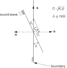
boundary from an orthogonal direction. But this is not always the case. Figure 1 shows a general example for plane waves in which the sound wave direction differs from
the boundary normal by an angle of .
Figure 1. A plane wave not normally incident to the boundary.
To consider this situation accurately, we adopt the plane-wave radiation equation used in
Sandler
(1998); that is,
where is the sound speed with and is the corresponding speed normal to the boundary. This exact description
of the geometry is the starting point for many developments of approximate absorbing
boundary conditions (see, for example, Engquist and
Majda, 1977). Thus, we have
Using the first-order expanding approximation to the second term in the square root in the
above equation (similar to what we did to reach Equation 45), we can obtain an improved radiation boundary condition
It can be found from comparison that this equation differs from Equation 46 only by a factor of for plane waves. In two dimensions the can be calculated as
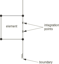
The normal and tangential derivatives and at the integration points can be evaluated using the corresponding element
along the radiation boundary surface (see Figure 2); that is,
where are the nodal pressure values of the element.
Figure 2. An element along the boundary.
The method described in this section can be used only for direct integration transient
dynamics; it cannot be used with steady-state or modal response. In addition, it is
available for planar, axisymmetric, and three-dimensional geometries.
Finally, the method makes the equilibrium equations nonlinear, as shown in Equation 52. Although in theory the iteration process in Abaqus/Standard can solve the nonlinear equilibrium equations accurately, the use of a small
half-increment residual tolerance is strongly suggested since in many cases the pressure and
its related residual along the radiation boundaries are very weak relative to the other
places in the modeled domain. The computation of at the integration point is based on the nodal pressures. The nodal
pressures are updated using the explicit central difference procedure described in Explicit dynamic analysis.