Interactions | ||
| ||
2025 GA
Step Cycling for Contact Wear Simulations
In many contact wear workflows, surface wear accumulates over thousands of physical wear cycles. It is often prohibitively expensive to simulate each physical wear cycle, so each simulated cycle typically represents a "batch" of multiple similar physical cycles. The animation below shows a wear simulation over five simulated cycles that represent 110,000 physical wear cycles in total. Step cycling allows the "batch size" to evolve during the simulation based on the maximum incremental wear distance in the simulated cycle. The number of simulated cycles is often not known before running such a simulation. For each simulated cycle, the user-specified wear coefficients are scaled by the current batch size.
The animation shows the wear distance accumulation on the slider and the bottom block as the slider repeatedly moves back and forth. In this example, the simulated wear cycle is modeled in two steps:
- In “Step-2” the slider moves to the right and returns to the center.
- In “Step-3” the slider moves to the left and returns to the center.
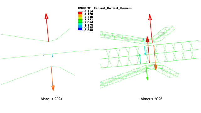
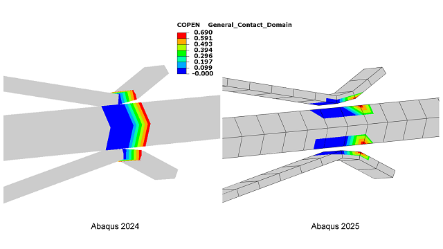
Contact Involving Beams with Noncircular Cross-Sections in Abaqus/Explicit
In earlier releases of Abaqus/Explicit, similar internally generated meshes could be used for simulations but they were not available for postprocessing. The following images compare plots of contact forces and contact opening distances on beam elements to plots on internally generated surface-element representations of the beams. Plots on surface elements show variations over the surfaces, similar to plots that would occur on the outer surface of a solid body, whereas plots based on beam elements are limited in that they represent a single value at each axial location.
Furthermore, some rounding of edges in the contact representation to improve numerics is achieved by offsetting nodes of internally generated surface elements inward and adding a small corresponding contact thickness. This contact thickness is not represented in plots, so the parts appear a bit smaller than the actual size.
2024 FD03
Arbitrary Lagrangian-Eulerian (ALE) Adaptive Meshing Supports Contact Wear in Abaqus/Explicit
The capability to simulate wear in general contact in Abaqus/Explicit was introduced in 2024 FD02. In that release Abaqus/Explicit treated the evolution of wear exclusively by considering nodal wear distances in contact penetration calculations. Now you can use arbitrary Lagrangian-Eulerian (ALE) adaptive meshing together with wear in Abaqus/Explicit to account for surface wear (erosion) in part geometries while preserving mesh quality, even for wear distances on the order of element dimensions.
The simulation on the left below shows the preexisting behavior (wear distances accounted for with offsets in contact penetration calculations). The simulation on the right demonstrates the use of ALE in the context of wear modeling. Similar wear accumulation occurs for both models, but it is much easier to interpret the wear configurations with ALE. Most wear occurs on the smaller block in this model, with the maximum wear distance being approximately half of the original element depth. In this example, ALE mesh smoothing effectively provides a realistic representation of the evolving part geometry while maintaining good mesh quality.

2024 FD02
Cohesive Contact in Abaqus/Explicit
Enhancements to cohesive contact in Abaqus/Explicit make cohesive contact a preferred alternative to surface-based tie constraints for modeling permanent, stiff bonds in more cases (for example, models where ties result in large implicit constraint systems or when you require interfacial traction results across connected surfaces).
Performance improvements for cohesive contact are most noticeable for models with a large fraction of nodes participating in cohesive contact. For example, simulations for the models shown in Figure 3 and Figure 4 with permanent, stiff cohesive contact bonds have sped up by 13% and 12%, respectively, compared to simulations in 2024 FD01.
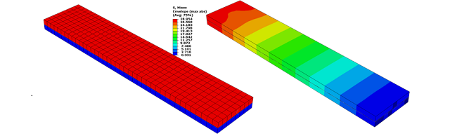
A second enhancement allows the default cohesive stiffness to be scaled by existing options to scale the contact penalty stiffness in Abaqus/Explicit. Cohesive contact, like other contact constraints, has a finite bond stiffness. You can assign the bond stiffness or allow it to take on the same contact penalty stiffness that would be in effect to resist penetrations for regular contact behavior, as discussed in Contact Cohesive Behavior. You can use a scale factor to increase the cohesive stiffness relative to the default value.
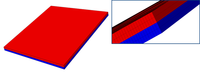
Figure 5 shows two blocks bonded together with
uniform tensile (negative pressure) loading of 1 × 10⁶ N/m2
applied to the top face of the top block while the bottom of the bottom block is
constrained. Loading is smoothly ramped on and damping is included to obtain a
quasi-static solution. 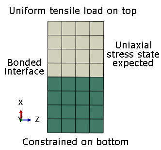


Alternatively, you can directly specify cohesive stiffness components, as discussed in Cohesive Stiffness. When you specify the cohesive stiffness, the penalty stiffness scale factor has no effect.
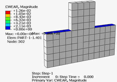
Contact Wear in Abaqus/Explicit
This new capability is available in Abaqus/Explicit for general contact analysis involving solid elements. Similar to the implementation introduced for Abaqus/Standard in 2024 FD01, the modeling approach accounts for local surface wear distances in contact penetration calculations but not in underlying element calculations.
The image below shows an example of accumulation of wear (shown as CWEAR contour
output) in a simplified helical bevel gear analysis. 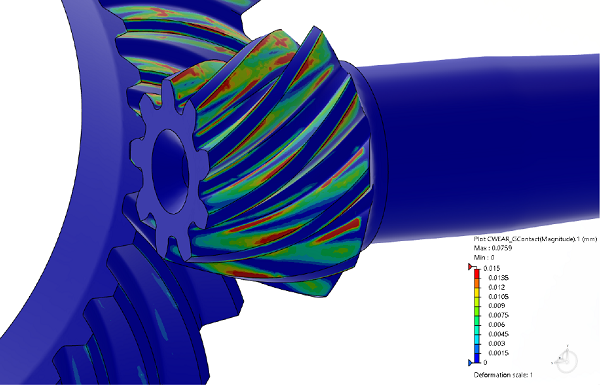
Usability enhancement for specifying reference thread geometry in Abaqus/Standard
Allowing reference thread geometry to be specified on either surface of a small-sliding interaction for general contact improves usability. Previously, this data was expected to be specified on whichever surface acting as the secondary surface of the contact formulation. However, main and secondary roles are typically left as default assignments for general contact in Abaqus/Standard, so a user typically would not know the secondary and main roles before running a simulation (and typically should not need to be aware of those roles).
The right side of Figure 8
shows that results in Abaqus 2024 HF2 are insensitive to whether reference thread geometry is specified for the
bolt or hole surface for small sliding interactions of general contact. In prior
versions, the expected behavior was obtained only if reference thread geometry was
specified for the secondary surface. 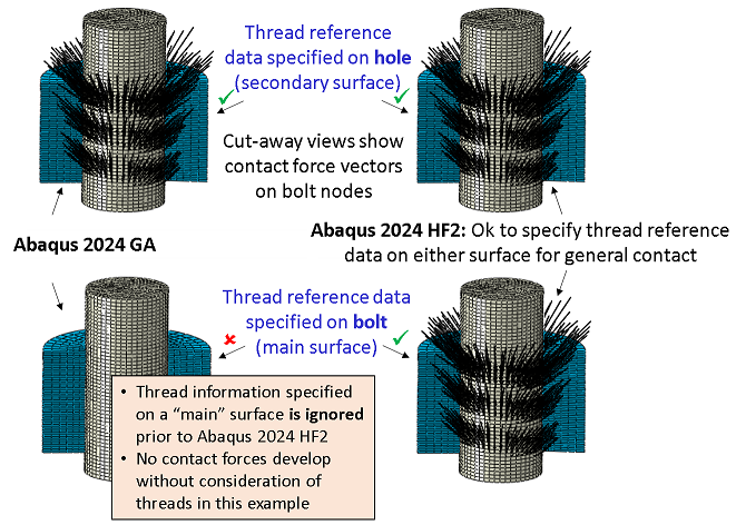
2024 FD01
Contact Wear in Abaqus/Standard
In many workflows, mechanical contact can cause wear on contacting surfaces due to mechanisms like abrasion and fretting. The new wear capability in Abaqus/Standard models wear evolution based on the Archard’s wear equation. Accordingly, contact nodal wear distances evolve based on wear properties of the surface material and on contact variables such as normal stress and slip distance. Abaqus/Standard treats wear distances as nodal offsets to the contact algorithm, resulting in a simplified approach to model wear fully within contact. It does not model the changes to geometry from wear explicitly. The approach considers the two-way physical influence of wear distance evolution on contact stresses (and underlying material stresses) and vice versa.
Figure 9 shows two blocks in contact. 
