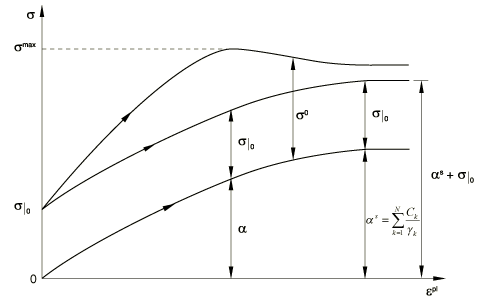
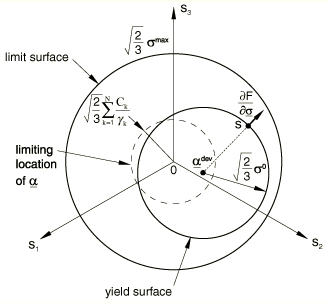
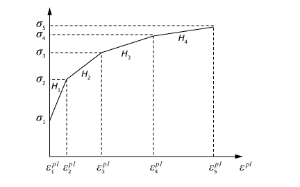
Models for metals subjected to cyclic loading

The total strain rate $\dot{\mathit{\epsilon }}$ is written in terms of the elastic and plastic strain rates as

The elastic behavior can be modeled only as linear elastic

where ${\mathbf{D}}^{el}$ represents the fourth-order elasticity tensor and $\mathit{\sigma }$ and $\mathit{\epsilon }$ are the second-order stress and strain tensors, respectively.

The models are pressure-independent plasticity models. For both the linear kinematic hardening model and the combined isotropic/kinematic hardening model, the yield surface is defined by the function

where $f\left(\mathit{\sigma }-\mathit{\alpha }\right)$ is the equivalent Mises stress or Hill's potential with respect to the backstress or “kinematic shift” $\mathit{\alpha }$ and ${\sigma }^0$ is the size of the yield surface. For example, the equivalent Mises stress is defined as

where ${\mathit{\alpha }}^{dev}$ is the deviatoric part of the backstress and $\mathbf{S}$ is the deviatoric stress tensor. Both of these models assume associated plastic flow:

where ${\dot{\mathit{\epsilon }}}^{pl}$ represents the rate of plastic flow and ${\dot{\overline{\epsilon }}}^{pl}$ is the equivalent plastic strain rate, ${\dot{\overline{\epsilon }}}^{pl}=\sqrt{\frac{2}{3}{\dot{\mathit{\epsilon }}}^{pl}:{\dot{\mathit{\epsilon }}}^{pl}}.$

In the multilinear kinematic hardening model, the response is assumed to be a weighted sum of various elastic-perfectly plastic elements. Each of these elements, also referred to as subvolumes, use the Mises yield surface with different yield strength. The flow rule for the multilinear kinematic hardening model is as follows:

where $N$ is the total number of subvolumes, $w_k$, $F_k$ , ${\dot{\overline{\epsilon }}}_k^{pl}$ and ${\sigma }_k$ are the weights, Mises yield surface, equivalent plastic strain rate, and the stress of the kth subvolume, respectively. Every subvolume follows an associated flow rule.

This model is the simplest of all the kinematic hardening models available in Abaqus. The size of the yield surface, ${\sigma }^0\left(\theta \right)$, can be a function of temperature only for this model. The evolution of $\mathit{\alpha }$ is defined by Ziegler's hardening rule, generalized to the nonisothermal case as

where $C\left(\theta \right)$ is the hardening parameter ($C\left(\theta \right)$ is the work-hardening slope of the isothermal uniaxial stress-strain response, $d\sigma /d{\overline{\epsilon }}^{pl}$, taken at different temperatures) and $\dot{C}$ is the rate of change of C with respect to time. This form of evolution law for $\mathit{\alpha }$ defines the rate of $\mathit{\alpha }$ due to plastic straining to be in the direction of the current radius vector from the center of the yield surface, $\mathit{\sigma }-\mathit{\alpha }$, and the rate due to temperature changes to be toward the origin of stress space. The inclusion of the $\dot{C}$ term in the evolution of $\mathit{\alpha }$ ensures that the material response is temperature history independent and, consequently, can be characterized with isothermal data. Rice (1975) writes this concept quite generally as

The particular identification of $\dot{\mu }=C{\dot{\overline{\epsilon }}}^{pl}/{\sigma }^0$ and $h=\left(dC/d\theta \right)/C$ in Equation 6 above is assumed, so the material behavior is defined by the isothermal, uniaxial work hardening data, $C\left(\theta \right)$ only.

This model is based on the work of Lemaitre and Chaboche (1990). The size of the yield surface, ${\sigma }^0\left({\overline{\epsilon }}^{pl},\theta ,f_i\right)$, is defined as a function of equivalent plastic strain, ${\overline{\epsilon }}^{pl}$; temperature, $\theta$; and field variables, $f_i$. This dependency can be provided directly, can be coded in user subroutine UHARD, or can be modeled with a simple exponential law for materials that either cyclically harden or soften as

where ${\sigma |}_0\left(\theta ,f_i\right)$ is the yield surface size at zero plastic strain, and $Q_{\mathrm{\infty }}\left(\theta ,f_i\right)$ and $b\left(\theta ,f_i\right)$ are additional material parameters that must be calibrated from cyclic test data.

The overall backstress is composed of multiple backstress components, where the evolution of the backstress components of the model is defined as

where

and the overall backstress is computed from the relation

where N is the number of backstresses; $C_k$, ${\gamma }_k$, ${\xi }_k$, ${\overline{R}}_k$, and $m_k$ are material parameters; and $\dot{C_k}$ is the rate of change of $C_k$ with respect to temperature and field variables. This equation is the basic Ziegler law, generalized to account for temperature and field-variable dependency of $C_k$ and to which a “recall” term, ${\gamma }_k{\mathit{\alpha }}_k{\dot{\overline{\epsilon }}}^{pl}$, and a static recovery term, ${\xi }_k{\left(\frac{\left|{\mathit{\alpha }}_k\right|}{{\overline{R}}_k}\right)}^{m_k-1}{\mathit{\alpha }}_k$, have been added. The recall term and the static recovery term introduce nonlinearity in the evolution law. The rate of change of ${\gamma }_k$ with respect to temperature and field variables is not accounted for in the evolution law for ${\mathit{\alpha }}_k$. Consequently, if ${\gamma }_k$ vary with temperature, the material response predicted by the model will be temperature history dependent. However, it can be shown that this dependency on temperature history is small and fades away with increasing plastic deformation. The condition for complete temperature history independent behavior is to use constant values for ${\gamma }_k$.

The evolution of the backstress and the isotropic hardening are illustrated in Figure 1 for unidirectional loading and in Figure 2 for multiaxial loading.

Figure 1. One-dimensional representation of the nonlinear model.

Figure 2. Three-dimensional representation of the nonlinear model.

The center of the yield surface is contained within a cylinder of radius $\sqrt{2/3}{\sum }_k^N{C}_k/{\gamma }_k$, which follows directly from Equation 10. Therefore, the yield surface is contained within the limiting surface of radius $\sqrt{2/3}{\sigma }^{max}$, as shown in the figures. This model can be degenerated into the linear kinematic model described above by setting ${\sigma }^0={\sigma |}_0$ and ${\gamma }_k=0$, for $k=1,\mathrm{\dots },N$.

The physical behavior that can be captured by this model, as well as its limitations, is described in detail in Models for Metals Subjected to Cyclic Loading.

The multilinear kinematic hardening model is defined by giving the value of uniaxial yield stress as a function of uniaxial plastic strain (Figure 3). The number of stress-plastic strain pairs given on the input curve determines the number of subvolumes, $N$, in the model. The yield strength of the kth subvolume (${\sigma }_{y,k}$) is calculated as

where (${\sigma }_k,{ϵ}_k^{pl}$) is the stress-plastic strain data provided by the user and $\mu$ is the shear modulus of the material. All the subvolumes are subjected to the same total strain, and the total stress is calculated as a weighted sum of stresses in the different subvolumes:

The weight of the kth subvolume is

where $H_k$is the hardening modulus between the kth data point and the $(k+1)$th data point on the stress versus plastic strain curve, defined by

The sum of weights over all subvolumes is one. It is assumed that the hardening modulus beyond the last data point is zero.

Figure 3. Uniaxial stress versus plastic strain curve in the case of the multilinear kinematic hardening model.