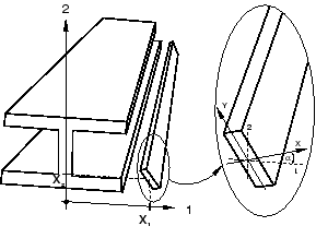
Defining a beam section's response to stretching, bending, shear,
and torsion of the beam's axis requires a suitable
definition of the axial force, N;
bending moments, and ; and torque, T, as
functions of the axial strain, ; curvature changes, and ; and twist, . Here the subscripts 1 and 2 refer to
local, orthogonal axes in the beam section.
If open-section beam types are used, the section behavior must also
define the warping bimoment,
W, and the generalized strain
measures include the warping amplitude,
w, and the
bicurvature of the
beam, , which is the gradient of the warping
amplitude with respect to position along the beam: .
The type of section definition you choose determines whether the
beam section properties are recomputed during the
progression of the analysis or established in the
preprocessor for the duration of the analysis. If a general
beam section definition is used (see Using a General Beam Section to Define the Section Behavior), the
cross-section properties are computed once, during
preprocessing. Alternatively, a beam section definition that
is integrated during the analysis can be used (see Using a Beam Section Integrated during the Analysis to Define the Section Behavior), in which
case Abaqus will use numerical integration of the stress over the
cross-section to define the beam's response as the analysis
proceeds.
Since planar beams deform only in the
X–Y
plane, only N and , and and , contribute to the response in these
elements: , , and w are assumed to
be zero.
In Abaqus bending moments in beam sections are typically measured
about the centroid of the beam section, while torque is
measured with respect to the shear center. In general, for
meshed beam sections that exhibit full coupling between the
strains, no unique centroid and shear center locations can
be defined. Therefore, all section forces and section
moments are given with respect to the beam axis for such
cross-sections. The beam axis (defined as the line joining
the nodes that define the beam element) need not pass
through the centroid of the beam section.
The degrees of freedom of the beam element are at the origin of the
local coordinate system defined in the
cross-section of the beam; that is, the line of the element
connecting the element's nodes passes through the origin of
the cross-section's local coordinate system.
Determining Whether to Use a Beam Section Integrated during the
Analysis or a General Beam Section
When a beam section integrated during the analysis is
used (see Using a Beam Section Integrated during the Analysis to Define the Section Behavior), Abaqus integrates numerically over the section as the
beam deforms, evaluating the material behavior
independently at each point on the section. This
type of beam section should be used when the
section nonlinearity is caused only by nonlinear
material response.
When a general beam section is used (see Using a General Beam Section to Define the Section Behavior), Abaqus precomputes the beam cross-section quantities
and performs all section computations during the
analysis in terms of the precomputed values. This
method combines the functions of beam section and
material descriptions. The precomputed section
properties might be specified in a variety of
ways, including quite complex geometries defined
with a two-dimensional finite element mesh (see
Meshed Beam Cross-Sections). A general beam
section should be used when the beam section
response is linear or when it is nonlinear and the
nonlinearity arises from more than just material
nonlinearity, such as in cases when section
collapse occurs.
Input File Usage
Use the following option to define a beam
section integrated during the analysis:
To define a beam section integrated during
the analysis:
Property module: Create Section: select Beam as the section Category and Beam as the section Type: Section integration: During analysis
To define a general beam section:
Property module: Create Section: select Beam as the section Category and Beam as the section Type: Section integration: Before analysis
Geometric Section Quantities
The section quantities described below are needed to define the
behavior of a general beam section.
Moments of Inertia
The moments of inertia with respect to the centroid are
defined as
where () is the position of the point in
the local beam section axis system and () is the position of the centroid
of the cross-sectional area.
Bending stiffness and rotary inertia contributions for a
meshed section profile (see Meshed Cross-Sections) are calculated using the two-dimensional
cross-section model. The following integrated
properties are defined for the entire
cross-section model meshed with 1-
DOF warping
elements:
where () is the center of mass of the
cross section.
Torsional Constant
The torsional constant, J, depends
on the shape of the cross section. The torsional
constant of a circular section is the polar moment
of inertia, .
The torsional constant for the rectangular and
trapezoidal library sections is calculated
numerically by Abaqus using the Prandtl stress function approach. A
local finite element model of the cross-section is
created internally for this purpose. The number of
integration points selected for the cross-section
determines the accuracy of this finite element
model. For increased accuracy specify a
higher-order rule by selecting nondefault
integration.
The above rule is also applied to both the thin-walled
box section and the arbitrary section to increase
the accuracy of the model. If the thickness for
each segment making up the section varies
significantly, more integration points for the box
section or smaller segments for the arbitrary
section should be specified in the area where the
thickness varies.
The torsional stiffness for a meshed section is
calculated over the two-dimensional region meshed
with 1-DOF
warping elements. The accuracy of the integration
depends on the number of elements in the
model:
where denotes the derivative of the
warping function with respect to the cross-section
(1, 2) axis and is the position of the shear
center of the cross-sectional area. All indices
take values 1, 2. For more details, see Meshed beam cross-sections.
For closed thin-walled sections the torsional constant is
calculated from
where t is the thickness of the
section, is the area enclosed by the
median line of the section, and
s is the length of the median
line, measured along the circumference of the
section in a counterclockwise direction.
For open, built-up, thin-walled sections,
Abaqus will check if a built-up section is closed or
not and will use the appropriate torsional
constant.
Sectorial Moment and Warping Constant
For open, thin-walled sections the sectorial moment is
defined as
and the warping constant is defined as
where is the sectorial area at a point
in the section with the shear center as its
pole.
Rotary Inertia for Timoshenko Beams
In general, the rotary inertia associated with torsional modes is
different from that of flexural modes. For unsymmetric
cross-sections the rotary inertia is different in each
direction of bending. For cross-sections where the beam node
is not located at the center of mass, coupling exists
between the translational and rotational degrees of
freedom.
By default, the exact (anisotropic and coupled) rotary inertia is
used for Timoshenko beams. In Abaqus/Standard the anisotropic rotary inertia introduces unsymmetric
terms in the Jacobian operator during geometrically
nonlinear, transient, direct-integration dynamic
simulations. If the rotary inertia effects are significant
in the geometrically nonlinear dynamic response and the
exact rotary inertia is used, the unsymmetric solver should
be used for better convergence.
Optionally, an approximate isotropic and uncoupled rotary inertia
can be selected. In Abaqus/Standard this means that the rotary inertia associated with the
torsional mode only is used for all rotational degrees of
freedom; potentially destabilizing rotary inertia effects in
impact problems due to the anisotropy or
displacement-rotation coupling will not be introduced. In
Abaqus/Explicit this means a scaled flexural inertia with a scaling
factor chosen to maximize the stable element time increment
is used for all rotational degrees of freedom; that is, the
stable time increment is not determined by the flexural
response of the beam. In some slender beam analyses an
isotropic approximation to the rotary inertia might be
accurate enough.
If beam elements are used to model plate-type structures in Abaqus/Explicit (that is, if the moment of inertia about one section axis
of the beam is more than a thousand times greater than the
moment of inertia about the other axis), the exact rotary
inertia formulation might lead to a sharp cut-back in the
stable time increment. In this case it is recommended that
you either use the isotropic approximation or alternatively
consider modeling the structure with shell elements, which
might be better suited to this type of analysis.
Isotropic rotary inertia for beam sections is not
supported in Abaqus/CAE. The default exact rotary inertia is always
used.
Adding Inertia to the Beam Section Behavior for Timoshenko Beams
You can define additional mass and rotary inertia properties for
Timoshenko beams (including
PIPE elements)
. This added inertia defined within the cross-section per
unit length along the beam contributes to the inertia
response of the beam without contributing to the structural
stiffness. However, you cannot define additional beam
inertia for a section if you use isotropic rotary inertia or
for beam elements with tapered cross-sections.
To specify additional beam inertia, you define the mass (per unit
length) with the mass center positioned at point in the local (1, 2) beam cross-section
axis system. To include rotary inertia (per unit length),
you can also define the angle (in degrees) within the cross-section
local (1, 2) system that positions the first axis of the
rotary inertia coordinate system relative to the local 1-direction in the
beam cross-section axis system. See Figure 1 for an illustration.
Figure 1. Beam element with added inertia.
The rotary inertia components relative to the rotary inertia
coordinate system are defined as
where A is the area, is the mass density, and
X and Y
are the local rotary inertia system coordinates measured
from , the center of the added mass
contribution.
As many point masses and rotary inertia contributions as are needed
to define the added inertia can be specified. Mass
proportional damping associated with the added inertia can
be specified by assigning a value to the mass proportional
Rayleigh damping coefficient, , or the composite damping coefficient, . Abaqus will use the mass weighted average (based on the material
damping and the added inertia damping) for the element mass
proportional damping.
Input File Usage
Use the following option in conjunction with the beam
section definition to specify additional inertia
properties:
Additional inertia properties are not supported in Abaqus/CAE.
Additional Inertia due to Immersion in Fluid
When a beam is fully or partially submerged, the effect of the
surrounding fluid can be modeled as an additional
distributed inertia on the beam (see Loading due to an incident dilatational wave field). By default, the beam
is assumed to be fully submerged. Alternatively, you can
specify that the added inertia per unit length should be
reduced by a factor of one-half to model a partially
submerged beam.
You specify the fluid mass density, (per unit volume); beam local
x and y
coordinates of the wetted cross-section centroid; wetted
section effective radius, r; and
empirical drag or flow coefficients, and . The inertia added per unit length to a
fully immersed beam cross-section is given by
Because the beam cross-section origin might not be coincident with
the centroid of the wetted cross-section, the additional
fluid inertia might include rotary effects. Nonzero values
for the x- and
y-offsets of the wetted cross-section
centroid will produce rotation-displacement coupling in the
inertia formulation. The default model for the added inertia
derives from inviscid flow around a cylindrical
cross-section (); you can specify a coefficient, , that models flow around a different
cross-section geometry.
An immersed beam also experiences an additional added mass effect
at its free ends. If a beam element's end node is not
attached to any other element and additional fluid inertia
is defined for this element, an additional mass might be
added in the form:
For this added mass corresponds to that of a
hemispherical cap; the default value is . The coefficient can be changed to model other geometries.
If the beam is partially submerged, the end inertia is
automatically reduced by one-half. However, the added mass
at the free ends is always isotropic: axial and transverse
motions experience the same additional inertia.
The virtual mass added to a submerged or partially
submerged beam is not included in the total mass, center of
mass, moments, or products of inertia reported in the data
(.dat) file.
Input File Usage
Use the following option in conjunction with the beam
section definition to define a fully immersed
beam: