Comparisons with equivalent beam MPC and equivalent
revolute and universal MPC problems show that using
coupling constraints yields identical behavior.
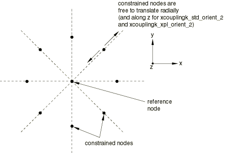
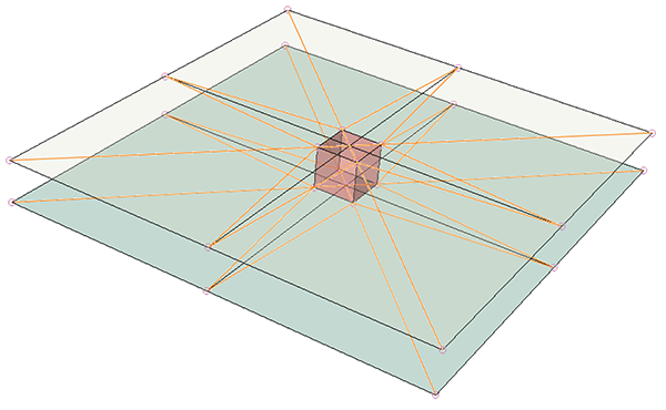
Figure 1. Geometry to test local orientation definitions.
In these tests the center node is the reference node, and the perimeter nodes are the
coupling nodes. Four separate coupling definitions that share the same reference node are
defined. Each coupling definition defines the local coordinate system using a different
orientation system: cylindrical, rectangular, spherical, and, for the Abaqus/Standard analyses, a system defined by user subroutine ORIENT. In all cases, the resulting
local constraint basis directions coincide with the local directions of a cylindrical
coordinate system whose axis is normal to the plane containing the nodes and passes
through the reference node.
In problems xcouplingk_std_orient_1.inp and xcouplingk_xpl_orient_1.inp the kinematic coupling
constrains all but the radial degree of freedom at the coupling nodes. Linear springs to
ground (SPRING1) for the Abaqus/Standard analyses and connector elements to ground
(CONN3D2) with linear elastic connector
behavior for the Abaqus/Explicit analyses are attached to all coupling nodes and act in the x- and
y-directions. The reference node is then rotated radians about the z-axis.
In problems xcouplingk_std_orient_2.inp and xcouplingk_xpl_orient_2.inpthe kinematic coupling
constrains the circumferential degree of freedom only. Linear springs to ground
(SPRING1) for the Abaqus/Standard analyses and connector elements to ground
(CONN3D2) with linear elastic connector
behavior for the Abaqus/Explicit analyses are attached to all coupling nodes and act in the x-,
y-, and z-directions. The reference node is then
rotated about x-axis.
Results and discussion
These tests result in motion of the constrained nodes, under action of the linear
springs, as the reference node rotates. For tests xcouplingk_std_orient_1.inp and xcouplingk_xpl_orient_1.inpthis motion remains on the
local radius passing through the node at all increments. For tests xcouplingk_std_orient_2.inp and xcouplingk_xpl_orient_2.inp this motion remains in
the plane defined by the original configuration local radius and the global
z-direction as this plane rotates according to the motion prescribed
at the reference node.
Test of local orientation and the release of two translational degrees of
freedom.
Internal sorting of kinematic coupling constraints
Features tested
The internal sorting of kinematic coupling constraints when used in conjunction with
MPC definitions is verified.
Problem description
The model consists of an axial arrangement of 20 shell elements. These elements are tied
together using a combination of kinematic coupling constraints as well as
MPCs. The constraints are defined such that the kinematic
coupling reference node appears after the constraint definitions that are eliminated
degrees of freedom on that node; thus, constraint sorting is required. The structure is
clamped on one end, and a concentrated axial load is applied on the other end.
Results and discussion
The test results in an internal sorting of kinematic coupling definitions and
MPCs so that the proper elimination order is achieved.
Test internal sorting of kinematic coupling constraints.
Distributing coupling constraints with user-specified weights
Features tested
The distributing coupling constraint is tested by using coupling and distributing
constraints with user-specified distributing weight factors. Geometric linear and
nonlinear tests are performed.
Problem description
Model:
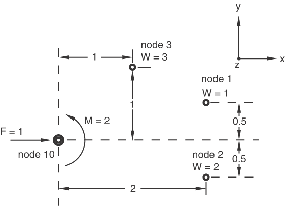
The initial starting geometry for each test is shown in Figure 2.
For the geometric linear test, for Abaqus/Standard, each coupling node is connected by a spring to ground
(SPRING1) in each direction. In the
geometrically nonlinear test in Abaqus/Standard, each coupling node is connected by a dashpot to ground
(DASHPOT1) in each direction, and an axial
spring element (SPRINGA) connects each
pair of coupling nodes. In the geometrically nonlinear test in Abaqus/Explicit, each coupling node is connected by a connector to ground
(CONN3D2) with damping behavior specified
in each direction, and a connector element with specified elastic behavior connects each
pair of coupling nodes. The reference node for the coupling constraint is node 10.
Figure 2. Initial starting geometry.
Linear behavior
Properties:
The spring stiffnesses are 100, 200, and 300 for degrees of freedom 1, 2, and
3, respectively, for the springs connected to all coupling nodes. The
distributing weight factors are 1, 2, and 3 for nodes 1, 2, and 3, respectively.
Loading:
Step 1
The force at the reference node is 1.0 in the
x-direction. The moment at the reference node is
2.0 about the z-axis.
Step 2
The force at the reference node is 1.0 in the
y-direction. The moment at the reference node is
2.0 about the x-axis.
Step 3
The force at the reference node is 1.0 in the
z-direction. The moment at the reference node is
2.0 about the y-axis.
Step 4
Frequency extraction.
Step 5
Transient modal dynamic step with a load, 1.0, applied to the reference node.
Step 6
Mode-based steady-state dynamic step with a load, 1.0, applied to the reference node.
Nonlinear behavior
Properties:
The dashpot damping coefficients are 100, 200, and 300 for degrees of freedom
1, 2, and 3, respectively, for the dashpots connected to all coupling nodes. The
axial springs connecting the coupling nodes each have a spring constant of 1.0 ×
108. The distributing weight factors are 1, 2, and 3 for nodes 1, 2,
and 3, respectively.
Prescribed reference node motion for Abaqus/Standard:
Step 1
Total rotation of about the z-axis. Translation .
Step 2
Total rotation of about the y-axis. Translation .
Step 3
Total rotation of about the x-axis. Translation .
Step 4
Direct-integration dynamic step with a total
rotation of about the z-axis. Translation .
Prescribed reference node motion for Abaqus/Explicit:
Step 1
Total rotation of about the z-axis. Translation .
Step 2
Total rotation of about the y-axis. Translation .
Step 3
Total rotation of about the x-axis. Translation .
Step 4
Total rotation of about the z-axis. Translation .
Results and discussion
In all tests the load distribution among coupling nodes adheres to the relation
where is the force distribution at the coupling nodes, and are the force and moment at the reference node, are the normalized distributing weight factors, is the coupling node arrangement inertia tensor, and and are the positions of the reference and coupling nodes relative to the
coupling node arrangement centroid, respectively. See Distributing coupling constraints for a more
detailed description of this load distribution.
Distributing coupling for geometric nonlinear case.
Default distributing weight factors
Elements tested
B21
B22
C3D8
C3D8R
C3D10M
C3D20
C3D27
CAX4
CAX4R
CAX8
CPE4
CPE4R
CPE8
S3R
S4
S8R
S9R5
CSS8
Features tested
The default distributing weight factors for a distributing coupling constraint are
verified. The weight factors are based on the nodal tributary surface area at each
coupling node.
Problem description
Various models consisting of either continuum, beam, or shell elements are used in this
test. In all models a uniform surface load is applied via a reference node and a
distributing coupling constraint. A nonuniform mesh density is used to verify that the
proper tributary area is calculated. The reference node is located at the center of the
loaded surface, offset in the normal direction.
Results and discussion
The displacements are equal to the displacements obtained if the model were loaded with a
uniform pressure load, hence verifying that the proper distributing weights are calculated
at the coupling nodes.
The calculation of distributing weights as outlined in Coupling Constraints when the
optional weighting method and influence region are specified is verified. The use of
coupling constraints at the part-instance level is also illustrated.
Problem description
A part is defined consisting of two rows of 20
CPE4R elements. Each element is a unit
square. The coupling nodes are defined along the top surface. A reference node is created
at the center of the top surface. The part is then instanced three times in the assembly
definition. For each part instance a coupling constraint with a different influence region
is defined. The first part instance has an infinite influence radius; that is, all nodes
defined on the surface will be included in the coupling definition. The second part
instance uses an influence radius of 5.5, and the third part instance uses an influence
radius of 0.5. A concentrated load is applied to each reference node. Input files are
provided for each weighting scheme: uniform, linear, quadratic, and cubic.
Results and discussion
The distributing weight factor calculations are verified to be according to the
description provided in Coupling Constraints. For the first
instance, all nodes belonging to the facets are included in the coupling definition. For
the second instance, the nodes of six facets adjacent to the reference node are included
in the coupling definition. In this case the facet farthest away from the reference node
(on either side) uses a facet participation factor of 0.5, since only part of element
surface facet is included in the influence region. For the third case, the nodes of the
adjacent facets to the reference node are included in the coupling definition. In this
case each facet has a participation factor of 0.5, since only part of the element surface
facet is included in the influence region.
Distributing coupling with a cubic weighting method.
Colinear coupling node arrangement
Features tested
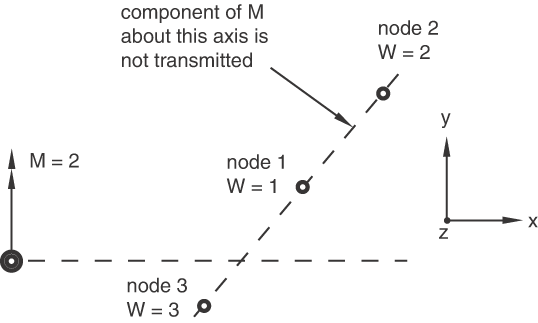
A pathological situation in which all coupling nodes are collinear for a distributing
coupling constraint and the moment applied at the reference node is not transmitted by the
constraint is tested.
The distributing coupling constraint connects a single reference node that has
translational and rotational degrees of freedom to a collection of coupling nodes that
have only translational degrees of freedom. Thus, when the coupling nodes are collinear in
a three-dimensional analysis, a situation can arise where the moments applied to the
reference node are not transmitted. In such a case Abaqus will print a warning message specifying the axis about which the moments are not
transmitted.
Distributing coupling with collinear coupling nodes.
Moment release for distributing coupling
Features tested
A series of linear and nonlinear analyses are performed demonstrating the ability of the
distributing coupling constraints to release the rotation constraints between the
reference node and the coupling nodes about user-specified axes.
Problem description
This example consists of both a two-dimensional and three-dimensional test.
In the two-dimensional test, two separate models are defined. Each model consists of a
single CPE4 element with one face coupled to
a reference node with a distributing constraint. The opposite face of the
CPE4 element is fixed. Beam elements are
attached to the reference nodes for visualization purposes only. The first model uses the
default coupling in which the rotation degree of freedom of the reference node is coupled
to the solid surface (the displacement degrees of freedom of the reference are always
coupled to the surface with distributing constraints). The second model releases the
rotation constraint. A series of boundary conditions are applied to the reference nodes
simulating shear, tension, and bending (in various linear and nonlinear steps).
In the three-dimensional test, eight separate models are defined. Each model consists of
a single C3D8 element with one face coupled
to a reference node with a distributing constraint. The opposite faces of the
C3D8 elements are fixed. Beam elements are
attached to the reference nodes for visualization purposes only. The first model uses the
default coupling in which all three rotation degrees of freedom of the reference node are
coupled to the solid surface. The next three models respectively release the rotation
constraint in the 1, 2, and 3 directions. The final four models are identical to the first
four, except that the rotation constraint directions are specified. A series of boundary
conditions are applied to the reference nodes simulating shear, tension, and bending (in
linear and nonlinear steps).
Results and discussion
The results clearly show that both coupling definitions in both two and three dimensions
are being applied properly.
Three-dimensional examples of distributing coupling with the moment constraints
released.
Dimensional coupling
Features tested
A series of linear analyses are performed demonstrating the ability of the distributing
coupling constraints to provide accurate dimensional coupling of beam elements to shell
and solid elements.
Problem description
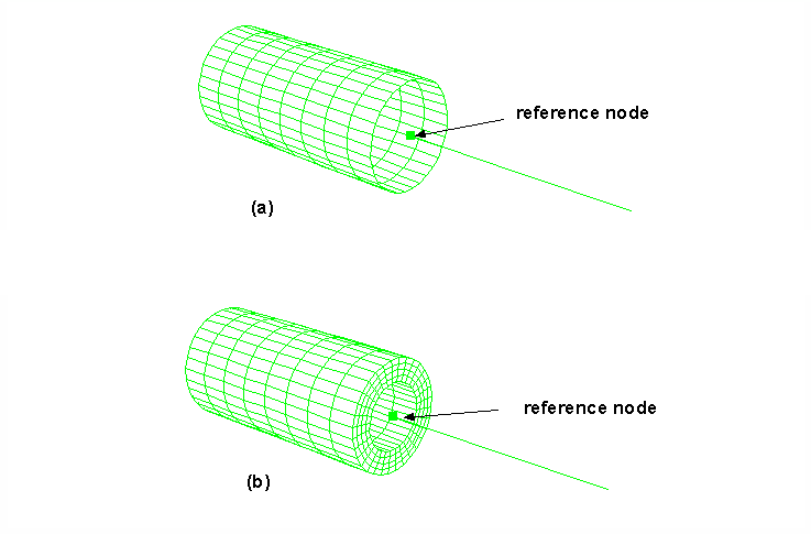
This example consists of two sets of tests in which a pipe is modeled with beam and shell
elements and with beam and continuum elements.
The pipe analyzed with beam and shell elements has a length of 0.8 m, an outside radius
of 0.1 m, and a thickness of 0.01 m. The material has a Young's modulus of 200 GPa and a
Poisson's ratio of 0.3. Half of the pipe is modeled with beam elements and the other half
is modeled with shell elements (see Figure 4(a)). The beam node closest to the shell model is defined as the reference node for the
distributing coupling constraint. An element-based edge surface is defined on the shell
model, which is coupled to the reference node. The coupled model is subjected to four
linear loading conditions simulating: (1) twist about the pipe axis, (2) axial stretch
along the pipe axis, (3) pure bending about the x-axis, and (4)
shear loading. The four load conditions are applied in a single linear step as four load
cases. Two models are analyzed: one with linear beam and shell elements and one with
quadratic beam and shell elements.
The pipe analyzed with beam and continuum elements has a length of 0.8 m, an outside
radius of 0.1 m, and a thickness of 0.04 m. The material has a Young's modulus of 200 GPa
and a Poisson's ratio of 0.3. Half of the pipe is modeled with beam elements and the other
half is modeled with continuum elements (see Figure 4(b)). The beam node closest to the continuum model is defined as the reference node for
the distributing coupling constraint. An element-based surface is defined on the continuum
model, which is coupled to the reference node. The coupled model is subjected to four
linear loading conditions simulating: (1) twist about the pipe axis, (2) axial stretch
along the pipe axis, (3) pure bending about the x-axis, and (4)
shear loading. The four load conditions are applied in a single linear step. Two models
are analyzed: one with linear beam and continuum elements and one with quadratic beam and
continuum elements.
Results and discussion
The resulting stress fields in the shell and solid models show minimal distortion at the
coupling interface, indication that the dimensional coupling is modeled accurately.
Coupling a beam model to a continuum model using quadratic beam and continuum
elements.
Structural coupling
Features tested
A series of analyses are performed demonstrating the structural coupling capability of
small distributing coupling constraints.
Problem description
Four different models, each with two small distributing couplings, are analyzed. In the
first model two small square plates are coupled together with a
BEAM connector. The connector nodes
are coupled to the two small surfaces using structural distributing couplings. One plate
is kept fixed, while the other is pulled upward (pried open) on one side. In the second
model, the same plates are pulled upward from all sides. In the third model two circular
plates are fastened together by placing a
BEAMMPC between the
reference nodes of two structural distributing couplings spanning two small patches on the
two plates. The plates are then subjected to relative shear motion. In the fourth model
two U-shaped shell specimens are connected in a fashion similar to that in the second
model. The lower specimen is fixed, while the upper specimen is lifted and pried open
simultaneously.
For comparison in Abaqus/Explicit, similar models are created to use continuum distributing coupling and fasteners.
Results and discussion
The resulting deformed shapes match the expectations. More important, if structural
coupling is used, contact between the plates does not occur in the area close to the
fastener, as expected. By contrast, contact does occur if continuum distributing couplings
are used.
Fourth model described above with structural coupling via fasteners.
Auto convert single facet distributing coupling to tie
Features tested
Abaqus/Explicit converts a distributing coupling to a
surface-based
tie constraint if the cloud nodes of the distributing coupling
correspond to a single facet of an element unless the reference node of the coupling is
connected to a connector element
Problem description
The model specifications involve distributing couplings with reference nodes
corresponding to nodes of solid elements and cloud nodes corresponding to nodes of shell
elements. Many of the distributed couplings specified in the model have cloud nodes
limited to one element face; Abaqus/Explicit automatically converts these distributed couplings to node-to-face surface-based tie
constraints involving the same set of nodes. The motivation for this conversion of the
model is that Abaqus/Explicit automatically adds mass to nodes that act as cloud nodes in multiple distributing
couplings, but Abaqus/Explicit does not automatically add mass to nodes acting as main nodes in multiple surface-based
tie constraints. Figure 5. A fastener construct involving a hexahedral element representing the faster
stiffness.
Results and discussion
Distributed couplings with cloud nodes associated with a single element face have been
internally converted to node-to-face surface-based tie constraints, and the amount of mass
artificially added to the model is reduced because fewer nodes participate in multiple
distributed couplings.