are used to simulate the inelastic behavior of materials that are subjected to cyclic
loading;
include a linear kinematic hardening model, a nonlinear isotropic/kinematic hardening
model, and, in Abaqus/Standard, a multilinear kinematic hardening model;
include a nonlinear isotropic/kinematic hardening model with multiple backstresses and,
optionally, static recovery effects;
can be used in any procedure that uses elements with displacement degrees of freedom;
in Abaqus/Standard cannot be used in adiabatic analyses;
can be used to model rate-dependent yield, except the multilinear kinematic hardening;
can be used with creep and swelling in Abaqus/Standard, except the multilinear kinematic hardening model; and
require the use of the linear elasticity material model to define the elastic part of the
response.
The kinematic hardening models used to model the behavior of metals subjected to cyclic
loading are pressure-independent plasticity models; in other words, yielding of the metals
is independent of the equivalent pressure stress. These models are suited for most metals
subjected to cyclic loading conditions, except voided metals.
The linear kinematic hardening model can be used with the Mises or Hill yield surface. The
nonlinear isotropic/kinematic model can be used only with the Mises yield surface in Abaqus/Standard and with the Mises or Hill yield surface in Abaqus/Explicit. The pressure-independent yield surface used in the linear kinematic hardening model and
the nonlinear isotropic/kinematic hardening model is defined by the function
where is the yield stress and is the equivalent Mises stress or Hill's potential with respect to the
backstress . For example, the equivalent Mises stress is defined as
where is the deviatoric stress tensor (defined as , where is the stress tensor, p is the equivalent pressure
stress, and is the identity tensor) and is the deviatoric part of the backstress tensor.
The response in the multilinear kinematic hardening model is assumed to be a weighted sum
of various elastic-perfectly plastic elements. Each of these elements, also referred to as
subvolumes, uses the Mises yield surface with a different yield strength.
Flow Rule
The kinematic hardening models assume associated plastic flow. The assumption of associated
plastic flow is acceptable for metals subjected to cyclic loading as long as microscopic
details, such as localization of plastic flow occurring as a metal component ruptures due to
cyclic fatigue loads, are not of interest.
Linear Kinematic Hardening Model and Nonlinear Isotropic/Kinematic Hardening
Model
In the case of the linear kinematic hardening model and the nonlinear
isotropic/kinematic hardening model:
where is the rate of plastic flow and is the equivalent plastic strain rate.
The evolution of the equivalent plastic strain is obtained from the following equivalent
plastic work expression:
which yields for isotropic Mises plasticity.
Multilinear Kinematic Hardening Model
The flow rule for the multilinear kinematic hardening model is as follows:
where is the total number of subvolumes and and are the weights, Mises yield surface, equivalent plastic strain rate,
and the stress of the kth subvolume, respectively. Every subvolume
follows an associated flow rule.
Hardening
The linear kinematic hardening model has a constant hardening modulus, and the nonlinear
isotropic/kinematic hardening model has both nonlinear kinematic and nonlinear isotropic
hardening components. The multilinear kinematic hardening model has a piecewise constant
hardening modulus.
Linear Kinematic Hardening Model
The evolution law of this model consists of a linear kinematic hardening component that
describes the translation of the yield surface in stress space through the backstress, . When temperature dependence is omitted, this evolution law is the
linear Ziegler hardening law
where is the equivalent plastic strain rate and C is the
kinematic hardening modulus. In this model the equivalent stress defining the size of the
yield surface, , remains constant, , where is the equivalent stress defining the size of the yield surface at zero
plastic strain.
Nonlinear Isotropic/Kinematic Hardening Model
The evolution law of this model consists of two components: a nonlinear kinematic
hardening component, which describes the translation of the yield surface in stress space
through the backstress, ; and an isotropic hardening component, which describes the change of the
equivalent stress defining the size of the yield surface, , as a function of plastic deformation.
The kinematic hardening component is defined to be an additive combination of a purely
kinematic term (linear Ziegler hardening law), a relaxation term (the
recall or dynamic recovery term), and, optionally, a static
recovery term. The last two terms introduce the nonlinearity. In addition, several
kinematic hardening components (backstresses) can be superposed, which may considerably
improve results in some cases. When temperature and field variable dependencies are
omitted, the hardening laws for each backstress are
where
and the overall backstress is computed from the relation
where is the number of backstresses, and , , , , and are material parameters that must be calibrated from cyclic test data. are the initial kinematic hardening moduli, and determine the rate at which the kinematic hardening moduli decrease with
increasing plastic deformation. , , and control the static recovery term. The kinematic hardening law can be
separated into a deviatoric part and a hydrostatic part; only the deviatoric part has an
effect on the material behavior. When , , and are zero, the model reduces to an isotropic hardening model. When all and equal zero, the linear Ziegler hardening law is recovered. Calibration
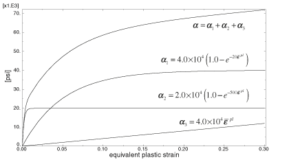
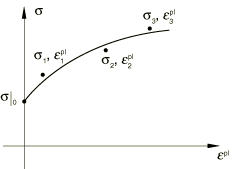
of the material parameters is discussed in Usage and Calibration of the Kinematic Hardening Models below. Figure 1 shows an example of nonlinear kinematic hardening with three backstresses.
Figure 1. Kinematic hardening model with three backstresses.
Each of the backstresses covers a different range of strains, and the linear hardening
law is retained for large strains.
The isotropic hardening behavior of the model defines the evolution of the yield surface
size, , as a function of the equivalent plastic strain, . This evolution can be introduced by specifying directly as a function of in tabular form, by specifying in user subroutine UHARD (in Abaqus/Standard only), or by using the simple exponential law
where is the yield stress at zero plastic strain and and b are material parameters. is the maximum change in the size of the yield surface, and
b defines the rate at which the size of the yield surface changes as
plastic straining develops. When the equivalent stress defining the size of the yield
surface remains constant (), the model reduces to a nonlinear kinematic hardening model.
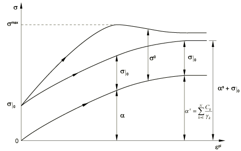
The evolution of the kinematic and the isotropic hardening components is illustrated in
Figure 2 for unidirectional loading and in Figure 3 for multiaxial loading. The evolution law for the kinematic hardening component implies
that the backstress is contained within a cylinder of radius , where is the magnitude of at saturation (large plastic strains). It also implies that any stress
point must lie within a cylinder of radius (using the notation of Figure 2) since the yield surface remains bounded. At large plastic strain any stress point is
contained within a cylinder of radius , where is the equivalent stress defining the size of the yield surface at large
plastic strain. If tabular data are provided for the isotropic component, is the last value given to define the size of the yield surface. If user
subroutine UHARD is used, this value will
depend on your implementation; otherwise, .
The model is applicable to strains up to about 25%–30%, and it is not recommended for
analyses in which these values are exceeded.
Figure 2. One-dimensional representation of the hardening in the nonlinear
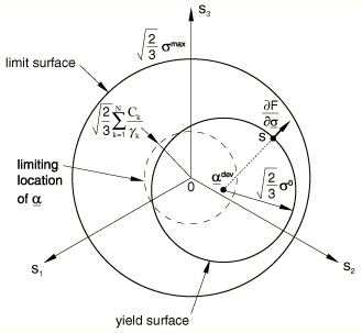
isotropic/kinematic model. Figure 3. Three-dimensional representation of the hardening in the nonlinear
isotropic/kinematic model.
Multilinear Kinematic Hardening Model
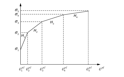
The multilinear kinematic hardening model is defined by giving the value of uniaxial
yield stress as a function of uniaxial plastic strain (Figure 4). The number of stress-plastic strain pairs given on the
input curve determines the number of subvolumes, , in the model. The yield strength of the kth
subvolume () is calculated as
where () is the user-specified stress-plastic strain data and is the shear modulus of the material. All the subvolumes are subjected
to the same total strain, and the total stress is calculated as a weighted sum of stresses
in the different subvolumes:
The weight of the kth subvolume is
where is the hardening modulus between the kth data point
and the (k +1)th data point on the stress versus plastic strain
curve. The sum of the weights over all the subvolumes is one. It is assumed that the
hardening modulus beyond the last data point is zero.
Figure 4. Uniaxial stress versus plastic strain curve in the case of the multilinear
kinematic hardening model.
Predicted Material Behavior
In the kinematic hardening models the center of the yield surface moves in stress space due
to the kinematic hardening component. In addition, when the nonlinear isotropic/kinematic
hardening model is used, the yield surface range may expand or contract due to the isotropic
component. These features allow modeling of inelastic deformation in metals that are
subjected to cycles of load or temperature, resulting in significant inelastic deformation
and, possibly, low-cycle fatigue failure. These models account for the following phenomena:
Bauschinger effect
This effect is characterized by a reduced yield stress upon load reversal after
plastic deformation has occurred during the initial loading. This phenomenon decreases
with continued cycling. The linear kinematic hardening component takes this effect
into consideration, but a nonlinear component improves the shape of the cycles.
Further improvement of the shape of the cycle can be obtained by using a nonlinear
model with multiple backstresses. The multilinear kinematic hardening model can also
be used to model this effect.
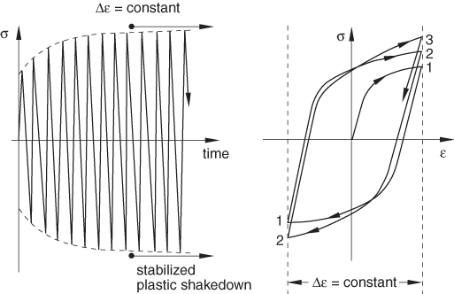
Cyclic hardening with plastic shakedown
This phenomenon is characteristic of symmetric stress- or strain-controlled
experiments. Soft or annealed metals tend to harden toward a stable limit, and
initially hardened metals tend to soften. Figure 5 illustrates the behavior of a metal that hardens under prescribed symmetric strain
cycles.
Figure 5. Plastic shakedown.
The kinematic hardening component of the models used alone predicts plastic shakedown
after one stress cycle. The combination of the isotropic component together with the
nonlinear kinematic component predicts shakedown after several cycles.
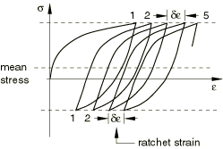
Ratchetting
Unsymmetric cycles of stress between prescribed limits will cause progressive “creep”
or “ratcheting” in the direction of the mean stress (Figure 6).
Figure 6. Ratchetting.
Typically, transient ratcheting is followed by stabilization (zero ratchet strain)
for low mean stresses, while a constant increase in the accumulated ratchet strain is
observed at high mean stresses. The nonlinear kinematic hardening component, used
without the isotropic hardening component, predicts constant ratchet strain. The
prediction of ratcheting is improved by adding isotropic hardening, in which case the
ratchet strain may decrease until it becomes constant. However, in general the
nonlinear hardening model with a single backstress predicts a too significant
ratcheting effect. A considerable improvement in modeling ratcheting can be achieved
by superposing several kinematic hardening models (backstresses) and choosing one of
the models to be linear or nearly linear (), which results in a less pronounced ratcheting effect. The
multilinear kinematic hardening model cannot predict this effect.
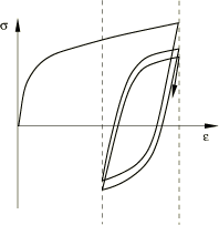
Relaxation of the mean stress
This phenomenon is characteristic of an unsymmetric strain experiment, as shown in
Figure 7.
Figure 7. Relaxation of the mean stress.
As the number of cycles increases, the mean stress tends to zero. The nonlinear
kinematic hardening component of the nonlinear isotropic/kinematic hardening model
accounts for this behavior.
Limitations
The linear kinematic model is a simple model that gives only a first approximation of the
behavior of metals subjected to cyclic loading, as explained above. The nonlinear
isotropic/kinematic hardening model can provide more accurate results in many cases
involving cyclic loading, but it still has the following limitations:
The isotropic hardening is the same at all strain ranges. Physical observations,
however, indicate that the amount of isotropic hardening depends on the magnitude of
the strain range. Furthermore, if the specimen is cycled at two different strain
ranges, one followed by the other, the deformation in the first cycle affects the
isotropic hardening in the second cycle. Thus, the model is only a coarse
approximation of actual cyclic behavior. It should be calibrated to the expected size
of the strain cycles of importance in the application.
The same cyclic hardening behavior is predicted for proportional and nonproportional
load cycles. Physical observations indicate that the cyclic hardening behavior of
materials subjected to nonproportional loading may be very different from uniaxial
behavior at a similar strain amplitude.
Usage and Calibration of the Kinematic Hardening Models
The linear kinematic model approximates the hardening behavior with a constant rate of
hardening. This hardening rate should be matched to the average hardening rate measured in
stabilized cycles over a strain range corresponding to that expected in the application. A
stabilized cycle is obtained by cycling over a fixed strain range until a steady-state
condition is reached; that is, until the stress-strain curve no longer changes shape from
one cycle to the next. The multilinear kinematic hardening model does not have the
restriction of a constant hardening rate. The more general nonlinear model will give better
predictions but requires more detailed calibration.
Linear Kinematic Hardening Model
The test data obtained from a half cycle of a unidirectional tension or compression
experiment must be linearized, since this simple model can predict only linear hardening.
The data are usually based on measurements of the stabilized behavior in strain cycles
covering a strain range corresponding to the strain range that is anticipated to occur in
the application. Abaqus expects you to provide only two data pairs to define this linear behavior: the yield
stress, , at zero plastic strain and a yield stress, , at a finite plastic strain value, . The linear kinematic hardening modulus, C, is
determined from the relation
You can provide several sets of two data pairs as a function of temperature to define the
variation of the linear kinematic hardening modulus with respect to temperature. If the
Hill yield surface is desired for this model, you must specify a set of yield ratios, , independently (see Hill Anisotropic Yield/Creep for
information on how to specify the yield ratios).
This model gives physically reasonable results for only relatively small strains (less
than 5%).
Property module: material editor: MechanicalPlasticityPlastic: Hardening: Kinematic
Nonlinear Isotropic/Kinematic Hardening Model
The evolution of the equivalent stress defining the size of the yield surface, , as a function of the equivalent plastic strain, , defines the isotropic hardening component of the model. You can define
this isotropic hardening component through an exponential law or directly in tabular form.
It need not be defined if the yield surface remains fixed throughout the loading. In Abaqus/Explicit if the Hill yield surface is desired for this model, you must specify a set of yield
ratios, , independently (see Hill Anisotropic Yield/Creep for
information on how to specify the yield ratios). The Hill yield surface cannot be used
with this model in Abaqus/Standard.
The material parameters and determine the kinematic hardening component of the model. Abaqus offers three different ways of providing data for the kinematic hardening component of
the model: the parameters and can be specified directly, half-cycle test data can be given, or test
data obtained from a stabilized cycle can be given. The experiments required to calibrate
the model are described below.
Optionally, you can include static recovery by specifying material parameters , , and . If you specify these parameters, all of the kinematic hardening
parameters must be specified directly. Test data input is not supported.
Defining the Isotropic Hardening Component by the Exponential Law
Specify the material parameters of the exponential law , , and b directly if they are already calibrated
from test data. These parameters can be specified as functions of temperature and/or
field variables.
Property module: material editor: MechanicalPlasticityPlastic: SuboptionsCyclic Hardening: toggle on Use parameters.
Defining the Isotropic Hardening Component by Tabular Data
Isotropic hardening can be introduced by specifying the equivalent stress defining the
size of the yield surface, , as a tabular function of the equivalent plastic strain, . The simplest way to obtain these data is to conduct a symmetric
strain-controlled cyclic experiment with strain range . Since the material's elastic modulus is large compared to its
hardening modulus, this experiment can be interpreted approximately as repeated cycles
over the same plastic strain range (using the notation of Figure 8, where E is the Young's modulus of the material).
Figure 8. Symmetric strain cycle experiment.
The equivalent stress defining the size of the yield surface is at zero equivalent plastic strain; for the peak tensile stress points
it is obtained by isolating the kinematic component from the yield stress (see Figure 2) as
for each cycle i, where . Since the model predicts approximately the same backstress value in
each cycle at a particular strain level, . The equivalent plastic strain corresponding to is
Data pairs (, ), including the value at zero equivalent plastic strain, are specified in tabulated form.
You should provide the tabulated values defining the size of the yield surface for the
entire equivalent plastic strain range to which the material may be subjected. You can
provide the data as functions of temperature and/or field variables. The yield stress at
a given state is interpolated from this table of data, and it is assumed to remain
constant outside the range of the independent variables other than equivalent plastic
strain. Outside the range of equivalent plastic strains, you can choose if the yield
stress remains constant (default) or is extrapolated linearly (see Extrapolation of Material Data).
To obtain accurate cyclic hardening data, such as would be needed for low-cycle fatigue
calculations, the calibration experiment should be performed at a strain range, , that corresponds to the strain range anticipated in the analysis
because the material model does not predict different isotropic hardening behavior at
different strain ranges. This limitation also implies that, even though a component is
made from the same material, it may have to be divided into several regions with
different hardening properties corresponding to different anticipated strain ranges.
Field variables and field variable dependence of these properties can also be used for
this purpose.
Abaqus allows the specification of strain rate effects in the isotropic component of the
nonlinear isotropic/kinematic hardening model. The rate-dependent isotropic hardening
data can be defined by specifying the equivalent stress defining the size of the yield
surface, , as a tabular function of the equivalent plastic strain, , at different values of the equivalent plastic strain rate, .
Input File Usage
Use the following option to define isotropic hardening with tabular data:
Property module: material editor: MechanicalPlasticityPlastic: Hardening: Combined: SuboptionsCyclic Hardening
Requesting linear extrapolation outside the specified range of the equivalent
plastic strains is not supported in Abaqus/CAE.
Defining the Isotropic Hardening Component in a User Subroutine in Abaqus/Standard
Specify directly in user subroutine UHARD. may be dependent on equivalent plastic strain and temperature. This
method cannot be used if the kinematic hardening component is specified by using
half-cycle test data.
You cannot define the isotropic hardening component in user subroutine UHARD in Abaqus/CAE.
Defining the Kinematic Hardening Component by Specifying the Material Parameters
Directly
The parameters and can be specified directly as a function of temperature and/or field
variables if they are already calibrated from test data. When depend on temperature and/or field variables, the response of the
model under thermomechanical loading will generally depend on the
history of temperature and/or field variables experienced
at a material point. This dependency on temperature-history is small and fades away with
increasing plastic deformation. However, if this effect is not desired, constant values
for should be specified to make the material response completely
independent of the history of temperature and field variables. The algorithm currently
used to integrate the nonlinear isotropic/kinematic hardening model provides accurate
solutions if the values of change moderately in an increment due to temperature and/or field
variable dependence; however, this algorithm may not yield a solution with sufficient
accuracy if the values of change abruptly in an increment.
The last term in the hardening law described in Nonlinear Isotropic/Kinematic Hardening Model above that is defined by the parameters , , and is called a static recovery term. This term allows you to capture the
stress relaxation when modeling material deformation at elevated temperatures.
Therefore, you should include this term if a model is subjected to loading at elevated
temperatures that includes strain holds, such as commonly performed cycling loading
tests with hold periods at tension and/or compression. If the static recovery term is
defined, it is active only in quasi-static, fully coupled temperature-displacement,
fully coupled thermal-electrical-structural, and implicit dynamic analyses.
Input File Usage
Use the following option to define hardening parameters if the static recovery
term is not included:
PLASTIC, HARDENING=COMBINED, DATA TYPE=PARAMETERS, NUMBER BACKSTRESSES=n
Use the following option to define hardening parameters if the static recovery
term is included:
PLASTIC, HARDENING=COMBINED, DATA TYPE=PARAMETERS, NUMBER BACKSTRESSES=n, STATIC RECOVERY
Abaqus/CAE Usage
Property module: material editor: MechanicalPlasticityPlastic: Hardening: Combined, Data type: Parameters, Number of backstresses: n
Including the static recovery term is not supported in Abaqus/CAE.
Defining the Kinematic Hardening Component by Specifying Half-Cycle Test
Data
If limited test data are available, and can be based on the stress-strain data obtained from the first half
cycle of a unidirectional tension or compression experiment. An example of such test
data is shown in Figure 9. This approach is usually adequate when the simulation will involve only a few cycles
of loading.
Figure 9. Half cycle of stress-strain data.
For each data point () a value of ( is the overall backstress obtained by summing all the backstresses at
this data point) is obtained from the test data as
where is the user-defined size of the yield surface at the corresponding
plastic strain for the isotropic hardening component or the initial yield stress if the
isotropic hardening component is not defined.
Integration of the backstress evolution laws over a half cycle yields the expressions
which are used for calibrating and .
When test data are given as functions of temperature and/or field variables, Abaqus determines several sets of material parameters (, ,..., , ), each corresponding to a given combination of temperature and/or
field variables. Generally, this results in temperature-history (and/or field
variable-history) dependent material behavior because the values of vary with changes in temperature and/or field variables. This
dependency on temperature-history is small and fades away with increasing plastic
deformation. However, you can make the response of the material completely independent
of the history of temperature and field variables by using constant values for the
parameters . This can be achieved by running a data check analysis first; an
appropriate constant values of can be determined from the information provided in the data file
during the data check. The values for the parameters and the constant parameters can then be entered directly as described above.
If the model with multiple backstresses is used, Abaqus obtains hardening parameters for different values of initial guesses and chooses the
ones that give the best correlation with the experimental data provided. However, you
should carefully examine the obtained parameters. In some cases it might be advantageous
to obtain hardening parameters for different numbers of backstresses before choosing the
set of parameters.
Static recovery is not available when you specify half-cycle test data.
Input File Usage
PLASTIC, HARDENING=COMBINED, DATA TYPE=HALF CYCLE, NUMBER BACKSTRESSES=n
Abaqus/CAE Usage
Property module: material editor: MechanicalPlasticityPlastic: Hardening: Combined, Data type: Half Cycle, Number of backstresses: n
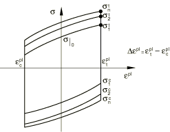
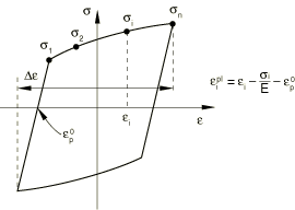
Defining the Kinematic Hardening Component by Specifying Test Data from a
Stabilized Cycle
Stress-strain data can be obtained from the stabilized cycle of a specimen that is
subjected to symmetric strain cycles. A stabilized cycle is obtained by cycling the
specimen over a fixed strain range until a steady-state condition is reached; that is, until the
stress-strain curve no longer changes shape from one cycle to the next. Such a
stabilized cycle is shown in Figure 10. Each data pair () must be specified with the strain axis shifted to , so that
and, thus, . In the above equation, denotes the total strain for data point , and .
Figure 10. Stress-strain data for a stabilized cycle.
For each pair () values of ( is the overall backstress obtained by summing all the backstresses at
this data point) are obtained from the test data as
where is the stabilized size of the yield surface.
Integration of the backstress evolution laws over this uniaxial strain cycle, with an
exact match for the first data pair (), provides the expressions
where denotes the backstress at the first data point (initial value of the backstress). The above equations enable calibration of the parameters and .
If the shapes of the stress-strain curves are significantly different for different
strain ranges, you may want to obtain several calibrated values of and . The tabular data of the stress-strain curves obtained at different
strain ranges can be entered directly in Abaqus. Calibrated values corresponding to each strain range are reported in the data file,
together with an averaged set of parameters, if model definition data are requested (see
Controlling the Amount of analysis input file processor Information Written to the Data File). Abaqus will use the averaged set in the analysis. These parameters may have to be adjusted
to improve the match to the test data at the strain range anticipated in the analysis.
When test data are given as functions of temperature and/or field variables, Abaqus determines several sets of material parameters (, ,..., , ), each corresponding to a given combination of temperature and/or
field variables. Generally, this results in temperature-history (and/or field
variable-history) dependent material behavior because the values of vary with changes in temperature and/or field variables. This
dependency on temperature-history is small and fades away with increasing plastic
deformation. However, you can make the response of the material completely independent
of the history of temperature and field variables by using constant values for the
parameters . This can be achieved by running a data check analysis first; an
appropriate constant values of can be determined from the information provided in the data file
during the data check. The values for the parameters and the constant parameters can then be entered directly as described above.
If the model with multiple backstresses is used, Abaqus obtains hardening parameters for different values of initial guesses and chooses the
ones that give the best correlation with the experimental data provided. However, you
should carefully examine the obtained parameters. In some cases it might be advantageous
to obtain hardening parameters for different numbers of backstresses before choosing the
set of parameters.
The isotropic hardening component should be defined by specifying the equivalent stress
defining the size of the yield surface at zero plastic strain, as well as the evolution
of the equivalent stress as a function of equivalent plastic strain. If this component
is not defined, Abaqus will assume that no cyclic hardening occurs so that the equivalent stress defining
the size of the yield surface is constant and equal to (or the average of these quantities over several strain ranges when
more than one strain range is provided). Since this size corresponds to the size of a
saturated cycle, this is unlikely to provide accurate predictions of actual behavior,
particularly in the initial cycles.
Static recovery is not available if you specify test data from a stabilized cycle.
Input File Usage
PLASTIC, HARDENING=COMBINED, DATA TYPE=STABILIZED, NUMBER BACKSTRESSES=n
Abaqus/CAE Usage
Property module: material editor: MechanicalPlasticityPlastic: Hardening: Combined, Data type: Stabilized, Number of backstresses: n
Multilinear Kinematic Hardening Model
The multilinear kinematic hardening model can be calibrated using the test data obtained
from a unidirectional tension or compression experiment. Abaqus expects you to provide the stress-plastic strain data pairs to define this multilinear
behavior. The hardening modulus between the kth data point and the th data point on the stress versus plastic strain curve, is determined from the relation
The data should be such that the hardening modulus does not increase with plastic strain.
The number of data points provided by the user determines the number of subvolumes, The computational cost and memory requirements increase with Therefore, the number of data points used to approximate the
stress-plastic strain curve with a piecewise linear response should always be minimized.
You can provide several sets of data pairs as a function of temperature and/or field
variable. However, you must ensure that the total number of data points or subvolumes
corresponding to different temperatures and/or field variables is the same.
Property module: material editor: MechanicalPlasticityPlastic: Hardening: Multilinear-Kinematic
Initial Conditions
When we need to study the behavior of a material that has already been subjected to some
hardening, Abaqus allows you to prescribe initial conditions for the equivalent plastic strain, , and for the backstresses, , in the case of the linear kinematic hardening model and the nonlinear
isotropic/kinematic hardening model. When the nonlinear isotropic/kinematic hardening model
is used, the initial conditions for each backstress, , must satisfy the condition
for the model to produce a kinematic hardening response. Abaqus allows the specification of initial backstresses that violate these conditions. However,
in this case the response corresponding to the backstress for which the condition is
violated produces kinematic softening response: the magnitude of the backstress decreases
with plastic straining from its initial value to the saturation value. If the condition is
violated for any of the backstresses, the overall response of the material is not guaranteed
to produce kinematic hardening response. The initial condition for the backstress has no
limitations when the linear kinematic hardening model is used.
You can specify the initial values of and directly as initial conditions (see Initial Conditions).
Load module: Create Predefined Field: Step: Initial, choose Mechanical for the Category and Hardening for the Types for Selected Step; Number of backstresses: n
User Subroutine Specification in Abaqus/Standard
For more complicated cases in Abaqus/Standard initial conditions can be defined through user subroutine HARDINI.
Load module: Create Predefined Field: Step: Initial, choose Mechanical for the Category and Hardening for the Types for Selected Step; Definition: User-defined, Number of backstresses: n
Elements
The linear kinematic hardening model and the nonlinear isotropic/kinematic hardening model
can be used with elements in Abaqus/Standard that include mechanical behavior (elements that have displacement degrees of freedom),
except some beam elements in space. Beam elements in space that include shear stress caused
by torsion (i.e., not thin-walled, open sections) and do not include hoop stress (i.e., not
PIPE elements) cannot be used with the
nonlinear kinematic hardening model. In Abaqus/Explicit, the linear kinematic hardening model and the nonlinear isotropic/kinematic hardening
model can be used with any elements that include mechanical behavior, with the exception of
one-dimensional elements (beams, pipes, and trusses) when the models are used with the Hill
yield surface. The multilinear kinematic hardening model can be used only in Abaqus/Standard with plane strain, generalized plane strain, axisymmetric, and three-dimensional solid
(continuum) elements.
Total kinematic hardening shift tensor components, .
ALPHAk
kinematic hardening shift tensor components ().
ALPHAN
All tensor components of all the kinematic hardening shift tensors, except the total
shift tensor.
PEEQ
Equivalent plastic strain, where is the initial equivalent plastic strain (zero or user-specified;
see Initial Conditions).
PENER
Plastic work, defined as: . This quantity is not guaranteed to be monotonically increasing for
kinematic hardening models. To get a quantity that is monotonically increasing, the
plastic dissipation needs to be computed as: . In Abaqus/Standard this quantity can be computed as a user-defined output variable in user subroutine
UVARM.