Rivets are a type of fastener designed to create permanent attachments between two or
more sheets of material. A rivet design typically consists of a cylindrical body
with two diameters: the smaller diameter is inserted through a hole in the
overlapping sheets, then both ends of the rivet are compressed. The compression
effectively expands the diameters of the rivet body, pinching the sheets of material
between the two ends of the rivet (see Figure 1). Different rivet designs and applications will undergo different deformations,
but the basic principle remains the same in all cases.
Three questions are of particular importance in this study:
Does the rivet deform appropriately during the forming process?
After the forming process, does the rivet retain enough strength to maintain
a hold on the fastened materials?
Is the rivet installation tool capable of forming the rivet?
The displacements during the forming simulation indicate whether or not the rivet
deforms appropriately. After the deformation, the strength of the rivet is based
largely on its material properties; examining the equivalent plastic strain in the
rivet gives some indication of potential damage or strength degradation in the
material. To assess the effect of the rivet on the installation tool, reaction
forces in the tool can be compared to known force capacities in standard
installation tools.
Geometry
The rivet used in these analyses is a simple multidiameter cylinder, as described
above. To aid the deformation of the smaller end of the rivet, a hemispherical
portion is removed from the center of the cylinder. Figure 2 shows the dimensions of the rivet model.
To simulate the forming, the rivet is placed in a hole at the center of a
circular plate. Circular dies representing the installation tool are positioned
at the top and bottom end of the rivet (see Figure 3).
Materials
The rivet in this model is composed of an elastic-plastic steel with a density of
7.85 × 10⁻⁹ t/mm3, Young's modulus of 2.1 × 10⁵
N/mm2, Poisson's ratio of 0.266, and the onset of plastic yielding
occurring at 3.0 × 10⁵ N/mm2.
The plate and dies are assumed to be significantly harder than the rivet, and no
deformation of these parts is expected.
Boundary conditions and loading
The forming process is simulated through the enforcement of displacement boundary
conditions. The plate is constrained to a fixed location. The top die is
displaced downward a distance of 3 mm, while at the same time the bottom die is
displaced upward a distance of 2 mm.
Interactions
Contact interactions must be enforced between the rivet and all installation tool
components; the deformation of the rivet depends on contact loads delivered
through the displacement of the tool. The tool components never come into
contact with each other, so interactions between the plate and dies can be
neglected.
Abaqus modeling approaches and simulation techniques
The rivet forming simulation is conducted in Abaqus/Explicit using two fundamentally different element formulations. The traditional
Lagrangian formulation generally offers accuracy and computational efficiency, but
pure Lagrangian models tend to exhibit mesh distortion and an associated loss of
accuracy when undergoing extreme deformations. The Eulerian formulation trades some
accuracy of geometry and results for robustness in analyses involving very large
deformations; in situations where the Lagrangian formulation yields an unreliable
solution or no solution at all, the Eulerian formulation can be used to obtain a
reasonable solution.
Lagrangian and Eulerian elements can be combined in the same model using a technique
known as coupled Eulerian-Lagrangian (CEL)
analysis. In a CEL analysis bodies that undergo
large deformations are meshed with Eulerian elements, while stiffer bodies in the
model are meshed with more efficient Lagrangian elements.
The rivet forming analysis is performed using both a pure Lagrangian approach, in
which the rivet, plate, and dies are all modeled with Lagrangian elements; and a
coupled Eulerian-Lagrangian approach, in which the rivet is modeled with Eulerian
elements while the plate and dies are modeled with Lagrangian elements.
The following sections detail some modeling techniques that are common to both
analysis cases.
Analysis Types
Both analysis cases are conducted using quasi-static explicit dynamic procedures.
The forming takes place over the course of a single step lasting 1 ms.
Materials
The material for the rivet uses an isotropic hardening Mises plasticity model.
The stress-strain data points used to define the plastic behavior are shown in
Table 1.
Boundary conditions
In both analysis cases the plate and dies are modeled as Lagrangian bodies
imposed with rigid body constraints. A boundary condition preventing
displacements and rotations is imposed on the reference point for the plate
body. Boundary conditions are also applied to each die reference point to
prevent them from rotating or displacing, except in the vertical 3-direction:
the boundary condition on the top reference point displaces it 3 mm in the
negative 3-direction, and the boundary condition on the bottom reference point
displaces it 2 mm in the positive 3-direction. The application of the boundary
conditions is governed by an amplitude that ramps the displacement linearly from
zero to full displacement over the course of 0.8 ms; the dies are then fixed in
place for the final 0.2 ms of the analysis.
Constraints
As mentioned above, rigid body constraints are applied to the plate and two dies.
These components are assumed to be significantly harder than the rivet, and they
do not deform during the forming process. The rigid body constraints improve
computational efficiency and allow the use of simple boundary conditions to
initiate the forming.
Output requests
Field output is specifically requested for the equivalent plastic strains in the
model (PEEQ). In addition,
history output for the reaction force in the 3-direction
(RF3) is requested at the
reference point for each of the dies.
Pure Lagrangian analysis case
The first analysis case uses four Lagrangian bodies meshed from discrete geometric
part instances. In the pure Lagrangian case the geometry of the model corresponds
directly to the shapes of the parts being modeled, making the assembly process
fairly intuitive.
Mesh design
The rivet is meshed with C3D8R
elements using a global mesh seed of 0.25 mm (see Figure 4).
The plate and dies are also meshed with
C3D8R elements, but the rigid body
constraints applied to these parts makes the element selection somewhat
arbitrary. Unmeshed analytical rigid surfaces could have been used to model the
plate and dies, but rigid body constraints are used to maintain consistency with
the CEL model.
Interactions
A general contact definition enforces contact interactions between all bodies in
the model. A frictionless, hard contact model governs all interactions.
Solution controls
Although large deformations are expected in the analysis, no special solution
controls or analysis techniques (such as adaptive meshing) are applied to the
model, allowing a straightforward comparison between the pure Lagrangian model
and the CEL model.
CEL analysis case
In the second analysis case the rivet is modeled using Eulerian elements. The plate
and dies are still rigid bodies. The modeling approach in the
CEL analysis has some distinct differences from the
pure Lagrangian case.
Mesh design
In the Eulerian formulation the mesh does not generally correspond to the
geometry of the part being modeled; rather, the placement of the material within
the Eulerian mesh defines the geometry of the part. The Eulerian mesh does not
deform or displace; only the materials within the mesh can move. Typically, the
Eulerian mesh is an arbitrary collection of regular hexahedral elements that
fully encompasses the region in which material might exist during the
analysis.
In this example the Eulerian part is a rectangular prism measuring 17 × 17 × 11.5
mm meshed with EC3D8R elements. A
global mesh seed of 0.25 mm dictates the element size.
This mesh does not define the geometry of the rivet; rather, the mesh defines the
domain in which the rivet material can exist. The rivet geometry is defined by
assigning steel material to a portion of this mesh corresponding to the shape of
the rivet, as discussed in the Initial conditions section below. One strength of
the Eulerian technique is the ability to define a regular, high-quality mesh
independent of the geometry of the part being modeled.
It is important that the Eulerian mesh is large enough to contain the rivet
material completely as it deforms; if material reaches the edge of the mesh, it
flows out of the model and is lost to the simulation.
Initial conditions
The rivet geometry is defined using a material assignment initial condition on
the Eulerian mesh. The material assignment specifies which elements in the mesh
initially contain steel. Each element is designated a percentage (known as the
volume fraction), which represents the portion of that element filled with
steel. For partially filled elements Abaqus positions the material in the element such that it forms a continuous surface
with the material in adjacent elements. The end result is a distribution of
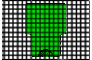
material in the mesh corresponding to the rivet geometry, as seen in Figure 5. You can use the view cut manager in the Visualization module of Abaqus/CAE to visualize the extent of a material within an Eulerian mesh, as discussed
in Viewing output from Eulerian analyses.
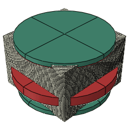
The material assignment is created with the aid of the volume
fraction tool in Abaqus/CAE. The volume fraction tool calculates the overlap between an Eulerian mesh and
some reference geometric part. To use the volume fraction tool for this analysis
case, the entire Lagrangian assembly (including the Lagrangian rivet) is copied
from the previous analysis case and positioned inside the Eulerian mesh (see
Figure 6). The Lagrangian rivet serves as the reference part, and the volume fraction
tool creates a discrete field that associates each element in the Eulerian mesh
with a volume fraction based on the amount of space occupied by the rivet within
that element. This discrete field can then be used as the basis for a material
assignment predefined field in Abaqus/CAE.
Interactions
A general contact definition enforces contact interactions between all rigid
bodies and Eulerian materials in the model. General contact does not enforce
contact between the rigid bodies and the Eulerian elements; the rigid bodies can
pass unimpeded through the Eulerian mesh until they encounter a material within
the mesh. As with the pure Lagrangian case, a frictionless, hard contact model
governs all interactions.
It is generally not advisable to model Lagrangian-Eulerian contact near the
boundary of the Eulerian mesh. The inflow or outflow of materials at the mesh
boundary can lead to improper contact constraint enforcement. Therefore, the
Eulerian mesh extends a few elements past the contact interfaces between the
dies and the rivet.
General contact does not enforce interactions between analytical rigid surfaces
and Eulerian materials, which is why the tool components must be modeled as
Lagrangian parts with rigid body constraints.
Output requests
In addition to the field and history output requests used in the pure Lagrangian
analysis case, the Eulerian volume fraction output variable
(EVF) is requested as field
output to visualize geometric results.
Discussion of results and comparison of cases
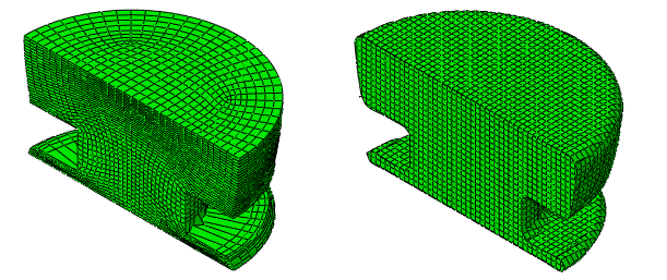
Figure 7 shows the deformed meshes for the pure Lagrangian and the
CEL analysis cases. (To view
the results of the CEL analysis, use the view cut
manager as described in Viewing output from Eulerian analyses.)
The pure Lagrangian analysis runs to completion, but the mesh becomes extremely
distorted along the bottom of the rivet—results from such an irregular mesh might be
unreliable. The Eulerian analysis exhibits a similar deformed shape but retains a
high-quality, regular mesh.
Computational efficiency
In general, an Eulerian analysis is more expensive than a comparable Lagrangian
analysis in terms of run times and file sizes. This performance tradeoff should
be weighed against the benefits of Eulerian robustness for large deformations
when choosing an analysis formulation.
Difficulties with contact
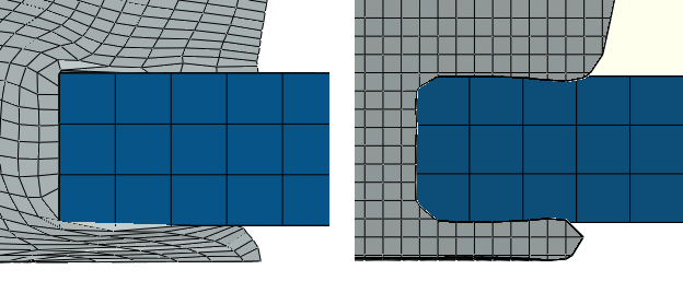
Figure 8 shows the contact interface between the rivet and the plate for both the pure
Lagrangian and the CEL cases. Both cases
demonstrate some undesirable penetration of the rivet into the plate.
In the pure Lagrangian case the penetrations are a direct result of mesh
distortion. As the rivet's facets spread out, there are fewer constraint points
per given area, and portions of the facets are able to pass unconstrained into
the plate surface. While the Lagrangian formulation is generally adept at
simulating contact, a severely deformed mesh can cause noisy, inconsistent
contact enforcement.
In the CEL case the penetrations result largely
from approximations used to visualize Eulerian material. The boundary of an
Eulerian material does not correspond to a discrete element face. As discussed
previously, Abaqus determines the location of material in an Eulerian mesh based on a volume
fraction within each element; the volume fractions are averaged and interpolated
to calculate a smooth material surface during visualization. Therefore, the material boundary displayed in the Visualization module of Abaqus/CAE is an approximation based on numerical averaging, not geometric properties.
The approximation causes the apparent penetrations at contact interfaces
and explains why sharp corners in a Lagrangian model appear rounded in an
Eulerian model. Despite the apparent penetrations, coupled Eulerian-Lagrangian
contact does not suffer from the inconsistent constraint enforcement associated
with pure Lagrangian mesh distortion, and contact between a solid Lagrangian
body and an Eulerian material typically delivers reliable results.
In both analysis cases contact penetrations can be alleviated through the use of
a finer mesh: smaller elements lead to reduced mesh distortion in the pure
Lagrangian case, and additional elements provide additional sample points for
more accurate volume fraction averaging in the Eulerian case.
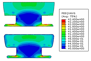
Interpreting results
A contour plot of the equivalent plastic strains in a cross-section of the
deformed rivet appears in Figure 9 for both analysis cases. The results are similar, but the regions of maximum
plastic strain occur in slightly different areas. In the Eulerian rivet the peak
strain occurs near the corner where the rivet meets the bottom of the plate;
this region undergoes extreme bending and stretching during the forming. In the
Lagrangian rivet the peak strain occurs in the elements with the most severe
distortion. For small to moderate deformation, the Eulerian approach provides
results that are comparable to the traditional Lagrangian approach (though at a
higher computational cost); for large deformation the Eulerian results appear
more reliable than the Lagrangian results.
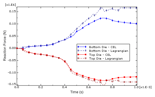
Figure 10
plots the reaction forces in both dies over the course of the forming process.
The results for the two formulations are comparable during the first half of the
analysis. However, the force plots for the pure Lagrangian analysis case exhibit
some noise during the latter half of the forming and subsequently diverge from
the Eulerian force plots. The noise is likely the result of contact difficulties
in the model (discussed above), which in turn lead to an uneven transfer of
force between the tooling and the rivet. After 0.8 ms, when the dies have fully
displaced, the forces in the Eulerian case exhibit some relaxation; the forces
in the Lagrangian case remain steadily higher than the corresponding Eulerian
forces due to the extreme deformation in the mesh.
Figure 1. Using a rivet to fasten two sheets of material. Figure 2. Rivet model geometry. All dimensions are in millimeters. Figure 3. Rivet assembled with the forming tools. All dimensions are in
millimeters. Figure 4. Rivet mesh in the pure Lagrangian case. Figure 5. Cross-section of the Eulerian mesh with the rivet material assigned. Figure 6. The Lagrangian parts are assembled inside of the Eulerian mesh. Figure 7. Deformed configuration for the pure Lagrangian case (left) and the
CEL case (right). Figure 8. Contact penetrations between the rivet and plate for the pure Lagrangian case
(left) and the CEL case (right). Figure 9. Equivalent plastic strain in the pure Lagrangian model (top) and the
CEL model (bottom). Figure 10. Reaction forces in the forming dies.