Sequential thermomechanical analysis of a directed energy deposition build
This example illustrates sequential thermomechanical analyses of directed
energy deposition builds of a thin-wall structure on a cantilevered substrate.
The
model in this problem is created based on published experiments (Denlinger et al., 2015). The
predicted results of temperature and distortions histories during printing are in good agreement
with experimental measurements.
This example demonstrates the following Abaqus features and techniques:
using temperature-dependent thermal and mechanical properties;
performing thermomechanical simulation of additive manufacturing processes, including
techniques of progressive element activation, progressive heating by a moving nonuniform heat
flux, and progressive cooling on evolving free surfaces; and
using special-purpose techniques for additive manufacturing.
Additive manufacturing (AM) technology has revolutionized
design and manufacturing. Directed energy deposition (DED)
is one of the common additive manufacturing technologies. During directed energy deposition,
the material is deposited by a nozzle mounted on a multi-axis arm and simultaneously melted
by a heat source (such as a laser or an electron beam). New material is added and solidifies
in a layer-by-layer fashion until the desired three-dimensional part is built.
This example problem simulates the fabrication of a thin-wall structure on a cantilevered
substrate using the directed energy deposition process (Denlinger et al., 2015). The test
setup consists of an aluminum clamp, a substrate, and a wall to be built on the center of
the substrate. The substrate and the wall are made of Inconel nickel-chromium alloy 625.
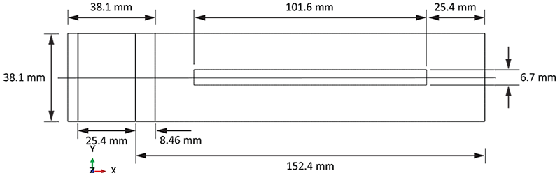
Geometry
As shown in Figure 1, the dimensions of the thin-wall structure are 101.6 mm (L)
× 6.7 mm (W) × 38.1 mm (H). The dimensions of the substrate are 152.4 mm (L) × 38.1 mm (W)
× 12.7 mm (H). The clamped region of the substrate is 8.46 mm long. The dimensions of the
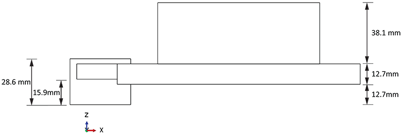
clamp are 38.1 mm (L) × 38.1 mm (W) × 28.6 mm (H).
Material deposition
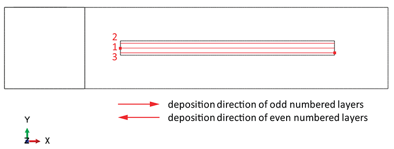
The wall is built using a three-bead deposition sequence per layer and a total of 42
layers. The in-plane material deposition motion is shown in Figure 2. For each layer, the center bead is deposited first,
followed by the two side beads. All beads in a layer are deposited in the same direction.
The deposition direction alternates between layers.
The travel speed of the nozzle is 10.6 mm/second. Thus, it takes 9.58 seconds to deposit
one bead. After the deposition of each bead, there is a cooling period of 4.66 seconds.
Three dwell times are considered for additional cooling after the deposition of each
layer: 0 seconds, 20 seconds, and 40 seconds.
The raw material (powder) is melted upon deposition by a laser with a power of 2 kW. The
laser beam spot size at the part surface is 4 mm in diameter. The penetration depth of the
laser is 1.1 mm.
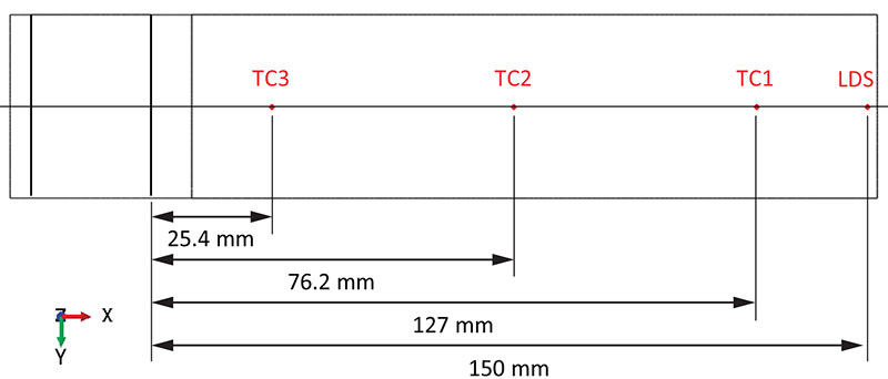
Experimental measurements
Temperature histories were measured during the printing process using three
thermocouples placed on the bottom of the substrate, away from the action zone. A laser
displacement sensor was used to measure the end deflection history of the substrate. Figure 3 shows the location of the thermocouples and the measurement
location of the displacement sensor.
Abaqus modeling approaches and simulation techniques
Three pairs of sequentially coupled thermomechanical analyses are performed in Abaqus/Standard to simulate three test cases of the Inconel builds of the thin-wall structure with
different interlayer dwell times.
Summary of analysis cases
Case 1
Sequential thermomechanical analysis of the build with
a 0 second interlayer dwell time
Case 2
Sequential thermomechanical analysis of the build with
a 20 second interlayer dwell time
Case 3
Sequential thermomechanical analysis of the build with
a 40 second interlayer dwell time
The following sections discuss analysis considerations that are applicable to all cases.
Analysis Types
A transient heat transfer analysis is performed first, considering thermal loads
introduced by the deposition process on the thin-wall structure. This analysis is followed
by a static structural analysis that is driven by the temperature field obtained by the
thermal analysis.
The wall mesh is progressively activated using full element activation (see Progressive Element Activation). The cross-section of a bead of material being deposited is
assumed to be rectangular with dimensions 3.35 mm (W) × 0.9071 (H), which is four elements
wide and one element high. The material deposition sequence is defined through an event
series.
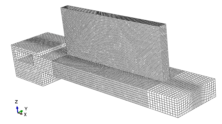
Mesh design
Figure 4 shows the finite element mesh of the model. The thin-wall
structure is modeled with a uniform mesh of 8-node linear brick elements. The element size
is 1.016 mm (L) × 0.838 mm (W) × 0.907 mm (H). A coarser mesh is used for the substrate
and the clamp. The heat transfer analysis and the structural analysis share the same mesh
strategy. DC3D8 elements are used in the
heat transfer analysis, and C3D8 elements
are used in the structural analysis.
Materials
The substrate and the wall are made of Inconel 625. The temperature-dependent thermal
conductivity, specific heat, the coefficient of thermal expansion, elastic modulus, and
yield stress are shown in Table 1 (Denlinger and Michaleris, 2016). The density is 8.44 ×
10-9 tonne/mm3. The solidus temperature is 1290°C, the liquidus
temperature is 1350°C, and the latent heat of fusion is 2.72 × 10¹¹ mJ/tonne.
The Poisson's ratio is 0.366.
The clamp is made of aluminum. Constant material properties are used:
Density
2.70 × 10⁻⁹ tonne/mm3
Conductivity
237 mW/(mm·°C)
Specific heat
9.1 × 10⁸ mJ/(tonne·°C)
Elastic modulus
70 × 103 MPa
Poisson's ratio
0.366
Coefficient of thermal expansion
2.31 × 10⁻⁵ /°C
Analysis steps
Each simulation is performed using three analysis steps. The deposition process is
modeled in the first step with a small time increment of 0.5 seconds. The second and the
third steps simulate additional cooling periods after the built with larger time
increments, 10 seconds and 100 seconds, respectively. The total time for cooling is 10,500
seconds.
Heat transfer analysis
Initial conditions
Newly deposited material comes in at room temperature, 26°C. The initial temperature of
the clamp and the substrate are also at room temperature.
Loads
A moving heat flux with a Goldak distribution is used to model the heating by the laser
upon deposition (see Specifying a Moving Heat Source with a Goldak Distribution). The laser beam spot at the intersection with the part
surface is assumed to be circular. The laser scanning path is defined through the same
event series that defines the material deposition sequence. The energy absorption
efficiency is calibrated to be 40% for all cases.
Nodal temperature (NT) field output is
requested for the whole model at every increment of the analysis for use in the subsequent
structural analysis. In addition, nodal temperature
(NT11) history output is requested for
the three nodes at the locations where the three thermocouples were placed in the
experiments.
Static structural analysis
Initial conditions
Based on the mesh size and the time incrementation used, the analyses presented in this
example can be categorized as part-level simulations of additive manufacturing processes.
To capture the melting effect in the structural analysis accurately, it is often necessary
to assign an initial temperature representing a relaxation temperature above which thermal
straining induces negligible thermal stress (see Controlling the Scale of the Simulation and the Solution Fidelity). In the structural analysis, the initial temperature of the
wall is set to the melting temperature of the material, 1290°C. The substrate and the
clamp are initially at the room temperature, 26°C.
Boundary conditions
All degrees of freedom of the nodes on the bottom and top surfaces of the clamp are
fixed.
Predefined fields
Nodal temperatures stored in the output database (.odb) file of the
previous transient heat transfer analysis are read as a predefined field. Abaqus automatically maps the nodal values of temperature by interpolation (both in space and
time) of the previous results.
Output requests
Nodal displacement (U), stress
(S),
strain(E), and equivalent plastic strain
(PEEQ) field output are requested for
the whole model. In addition, nodal displacement
(U3) history output is requested for the
node at the location where the deflection of the substrate was measured in the
experiments.
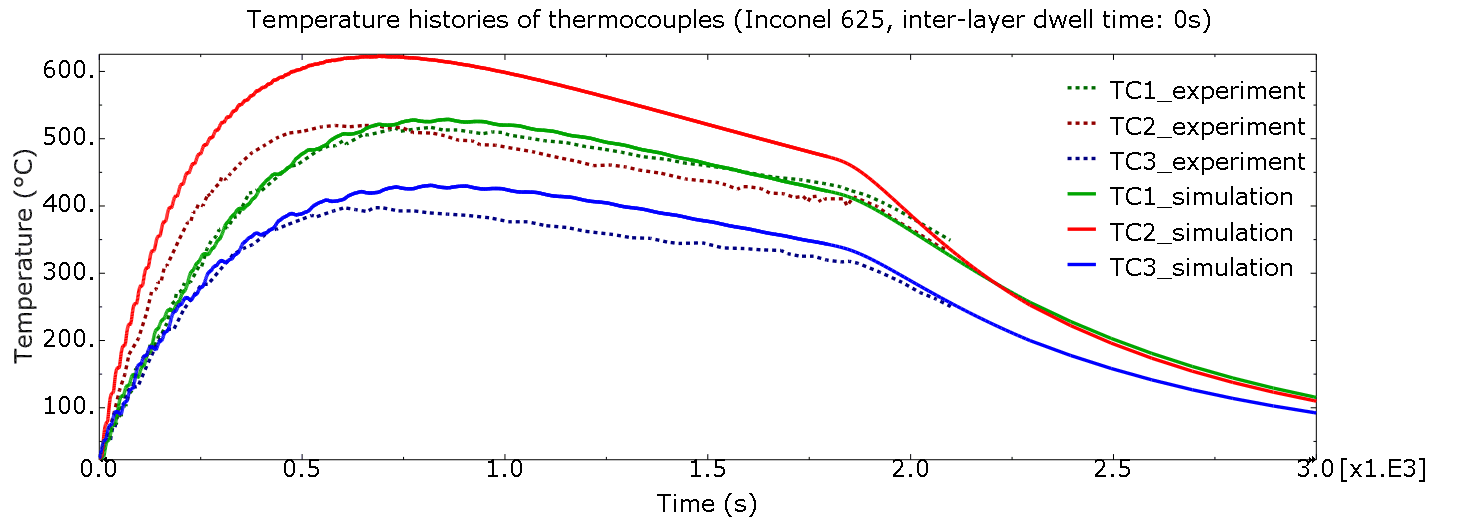
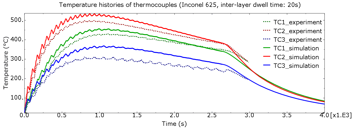
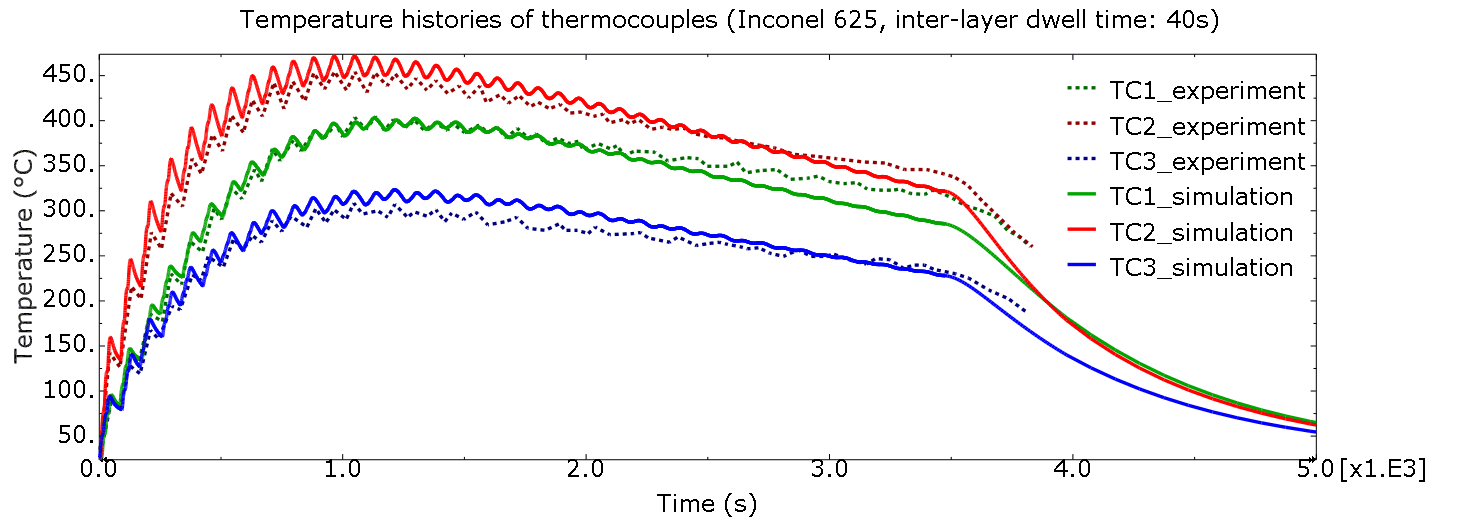
Discussion of results and comparison of cases
As shown in Figure 5, the simulations of the temperature histories of the three
locations on the bottom of the substrate agree well with the in-situ experimental
measurements for all cases. The agreement in temperature histories at locations that are
away from the action zone indicates that the heat energy balance of the system, including
heat energy input by the laser, thermal conduction, and cooling by convection and radiation,
is well captured.
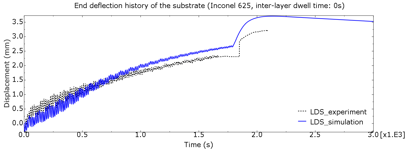
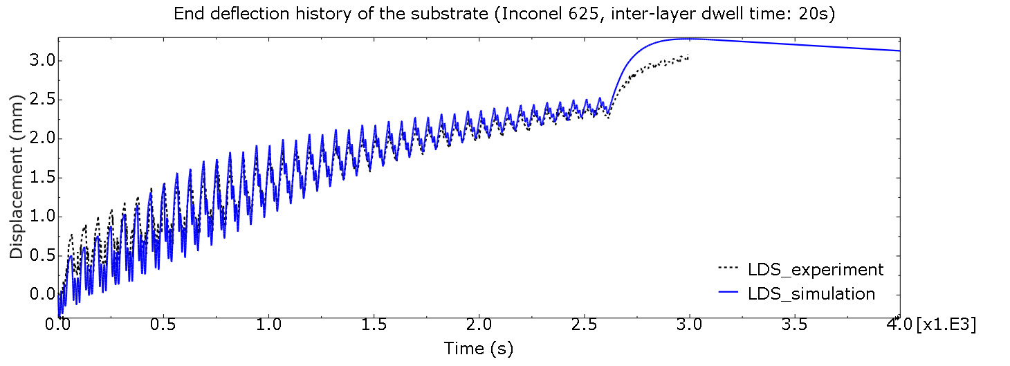
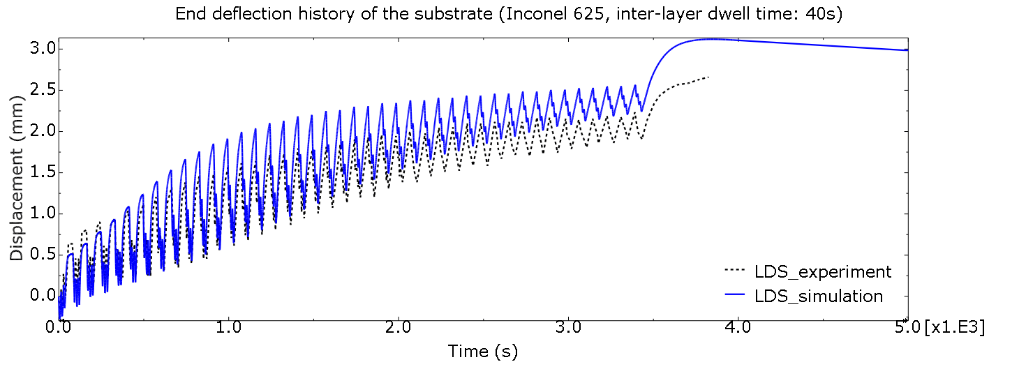
Figure 6 compares the simulated and measured deflections of the free
end of the substrate for all cases. The oscillation due to the alternating deposition and
cooling periods and the accumulated deflection of the substrate are well captured. The
substrate bends downward during deposition due to a larger thermal expansion of the top
surface relative to the bottom surface, while it bends upward during the cooling period
because the substrate cools down and the deposited material also starts to contract
(Denlinger et al., 2015). The final distortion and residual stresses of the substrate are
caused primarily by the thermal contraction of the thin-wall structure.
Types of property tables, parameter tables, and event series used by the
special-purpose techniques for the simulation of common additive manufacturing
processes in Abaqus.
Event series data of the material deposition (and laser scanning)
motion, used by the analyses of the builds with a 40 second interlayer dwell
time.
References
Denlinger, E.R., J. C. Heigel, P. Michaleris, and T. A. Palmer, "Effect of Inter-layer Dwell Time on Distortion and
Residual Stress in Additive Manufacturing of Titanium and Nickel Alloys,"
Journal of Materials Processing
Technology, vol. 215, pp. 123–131, 2015.
Denlinger, E.R., , and P. Michaleris, "Effect of Stress Relaxation on Distortion in Additive
Manufacturing Process Modeling," Additive
Manufacturing, vol. 12, pp. 51–59, 2016.
Tables
Table 1. Temperature-dependent material properties of Inconel 625 (Denlinger and Michaleris,
2016).
Temperature (°C)
Conductivity (mW/(mm·°C))
Specific Heat (mJ/(tonne·°C))
Coefficient of Thermal Expansion (1/°C)
Elastic Modulus (MPa)
Yield Stress (MPa)
20
9.9
4.10 × 10⁸
1.28 × 10⁻⁵
2.08 × 10⁵
493
93
10.8
4.27 × 10⁸
1.28 × 10⁻⁵
2.04 × 10⁵
479
205
12.5
4.56 × 10⁸
1.31 × 10⁻⁵
1.98 × 10⁵
443
315
14.1
4.81 × 10⁸
1.33 × 10⁻⁵
1.92 × 10⁵
430
425
15.7
5.11 × 10⁸
1.37 × 10⁻⁵
1.86 × 10⁵
424
540
17.5
5.36 × 10⁸
1.40 × 10⁻⁵
1.79 × 10⁵
423
650
19.0
5.65 × 10⁸
1.48 × 10⁻⁵
1.70 × 10⁵
422
760
20.8
5.90 × 10⁸
1.53 × 10⁻⁵
1.61 × 10⁵
415
870
22.8
6.20 × 10⁸
1.58 × 10⁻⁵
1.48 × 10⁵
386
Figures
Figure 1. Dimensions (Denlinger et al., 2015).
Figure 2. The material deposition (and laser scanning) path (Denlinger et al., 2015). Figure 3. Locations of the thermocouples (TC) and the
measurement location of the laser displacement sensor
(LDS) on the bottom of the substrate (Denlinger et al.,
2015). Figure 4. Finite element mesh. Figure 5. Temperature histories of thermocouples.
Figure 6. End deflection histories of the substrate.