X–Y plotting

You can create X–Y curves from either history or field data stored in the output database (.odb) file. X–Y curves can also be read from an external file or they can be typed into the Visualization module interactively. Once curves have been created, their data can be further manipulated and plotted to the screen in graphical form.

The X–Y plotting capability of the Visualization module is discussed further in Materials.

Context:

You saved the displacements of the midspan nodes (node set Midspan) in the history portion of the output database file NlSkewPlate.odb for each increment of the simulation. You can use these results to create X–Y plots. In particular, you will plot the vertical displacement history of the nodes located at the edges of the plate midspan.
  1. First, display only the nodes in the node set named Midspan: in the Results Tree, expand the Node Sets container underneath the output database file named NlSkewPlate.odb. Click mouse button 3 on the set named MIDSPAN, and select Replace from the menu that appears.
  2. Use the Common Plot Options dialog box to show the node labels (i.e., numbers) to determine which nodes are located at the edges of the plate midspan.
  3. In the Results Tree, expand the History Output container for the output database named NlSkewPlate.odb.
  4. Locate the output labeled as follows: Spatial displacement: U3 at Node xxx in NSET MIDSPAN. Each of these curves represents the vertical motion of one of the midspan nodes.
  5. Select (using CtrlClick) the vertical motion of the two midspan edge nodes. Use the node labels to determine which curves you need to select.
  6. Click mouse button 3, and select Plot from the menu that appears.

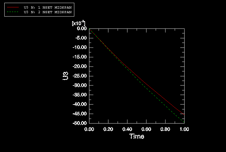
    Abaqus reads the data for both curves from the output database file and plots a graph similar to the one shown in Figure 1. (For clarity, the second curve has been changed to a dashed line, and the default grid and legend positions have been changed.)

    Figure 1. Midspan displacement history at the edges of the skew plate.

    The nonlinear nature of this simulation is clearly seen in these curves: as the analysis progresses, the plate stiffens. In this simulation the increase in the plate stiffness with the deformation is due to membrane effects. Therefore, the resulting peak displacement is less than that predicted by the linear analysis, which did not include this effect.