For the static linear perturbation analysis done in
Abaqus/Standard
you examined the deformed shape as well as stress, displacement, and reaction
force output. For the
Abaqus/Explicit
analysis you can similarly examine the deformed shape and generate field data
reports.
Because this is a dynamic analysis, you should also examine the
transient response resulting from the loading. You will do this by animating
the time history of the deformed model shape and plotting the displacement
history of the bottom center node in the truss.
Plot the deformed shape of the model. For large-displacement analyses (the
default formulation in
Abaqus/Explicit)
the displaced shape scale factor has a default value of 1. Change the
Deformation Scale Factor to 20 so that you can more easily
see the deformation of the truss.
Create a time-history animation of the deformed model shape
From the main menu bar, selectAnimateTime
History; or use the
tool in the toolbox.
The time history animation begins in a continuous loop at its fastest
speed.
Abaqus/CAE
displays the movie player controls in the right side of the context bar
(immediately above the viewport).
From the main menu bar, selectOptionsAnimation;
or use the animation options
tool in the toolbox (located directly underneath the
tool).
The Animation Options dialog box appears.
Change the Mode to Play
Once, and slow the animation down by moving the Frame
Rate slider.
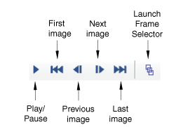
You can use the animation controls to start, pause, and step through
the animation. From left to right of
Figure 1,
these controls perform the following functions:
play/pause, first,
previous, next, and
last.
Figure 1. Postprocessing animation controls.
Create an X–Y plot of the vertical displacement for
a node
Context:
The truss responds dynamically to the load. You can confirm this by plotting
the vertical displacement history of the node set
Center.
You can create X–Y curves from either history or field
data stored in the output database (.odb) file.
X–Y curves can also be read from an external file or they
can be typed into the Visualization module interactively. Once curves have been
created, their data can be further manipulated and plotted to the screen in
graphical form. In this example you will create and plot the curve using
history data.
In the
Results Tree,
expand the History Output container underneath the output
database named expFrame.odb.
From the list of available history output, double-click
Spatial displacement: U2 at Node x
		in NSET CENTER
.
Abaqus/CAE
plots the vertical displacement at the center node along the bottom of the
truss, as shown in
Figure 2.
Figure 2. Vertical displacement at the midspan of the truss.
Note:
The chart legend has been suppressed and the axis
labels modified in this figure. Many X–Y plot
options are directly accessible by double-clicking the appropriate regions of
the viewport. To enable direct object actions, however, you must first click
in the prompt area to cancel the current procedure (if
necessary). To suppress the legend, double-click it in the viewport to open the
Chart Legend Options dialog box. In the
Contents tabbed page of this dialog box, toggle off
Show legend. To modify the axis labels, double-click
either axis to open the Axis Options dialog box, and edit
the axis titles as indicated in
Figure 2.
Exiting
Abaqus/CAE
Save your model database file; then select
FileExit
from the main menu bar to exit
Abaqus/CAE.
 tool in the toolbox.
 tool in the toolbox (located directly underneath the

 in the prompt area to cancel the current procedure (if
necessary). To suppress the legend, double-click it in the viewport to open the
in the prompt area to cancel the current procedure (if
necessary). To suppress the legend, double-click it in the viewport to open the