Postprocessing | ||
| ||
The Visualization module automatically uses the last available frame on the output database file. The results from the second step of this simulation are the natural mode shapes of the pipe and the corresponding natural frequencies. Plot the first mode shape.
- From the main menu bar, select
.
The Step/Frame dialog box appears.
- Select step Frequency I and frame Mode 1.
- Click .
- From the main menu bar, select .
- Click the
 tool in the toolbox to allow multiple plot states in the viewport,
then click the
 tool or select
to add the undeformed shape plot to the
existing deformed plot in the viewport.
 - Include node symbols on both plots (the superimpose options control the appearance of the undeformed shape when multiple plot states are displayed). Change the color of the node symbols to green and the symbol shape to a solid circle.
- Click the auto-fit tool
 so that the entire plot is rescaled to fit in the
viewport.
The default view is isometric. Try rotating the model to find a better view
of the first eigenmode, similar to that shown in
Figure 1.

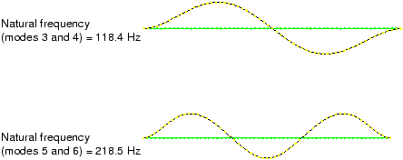
Since this is a linear perturbation step, the undeformed shape is the shape of the structure in the base state. This makes it easy to see the motion relative to the base state. Use the Frame Selector to plot the other mode shapes. You will discover that this model has many repeated eigenmodes. This is a result of the symmetric nature of the pipe's cross-section, which yields two eigenmodes for each natural frequency, corresponding to the 1–2 and 1–3 planes. The second eigenmode shape is shown in Figure 1. Some of the higher vibrational mode shapes are shown in Figure 2.

The natural frequency associated with each eigenmode is reported in the plot title. The lowest natural frequency of the pipe section when the 4 MN tensile load is applied is 47.1 Hz. The tensile loading has increased the stiffness of the pipe and, thus, increased the vibrational frequencies of the pipe section. This lowest natural frequency is within the frequency range of the harmonic loads; therefore, resonance of the pipe may be a problem when it is used with this loading.
You, therefore, need to continue the simulation and apply additional tensile load to the pipe section until you find the magnitude that raises the natural frequency of the pipe section to an acceptable level. Rather than repeating the analysis and increasing the applied axial load, you can use the restart capability in Abaqus to continue the load history of a prior simulation in a new analysis.