Modifications to the model | ||
| ||
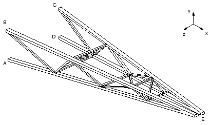
The connections at points A, B, C, and D (see Figure 1) can only withstand a maximum pull-out force of 100 kN. You have to decide whether or not any of these connections will break.

The short duration of the loading means that inertia effects are likely to be important, making dynamic analysis essential. You are not given any information regarding the damping of the structure. Since there are bolted connections between the trusses and the cross bracing, the energy absorption caused by frictional effects is likely to be significant. Based on experience, you therefore choose 5% of critical damping in each mode.
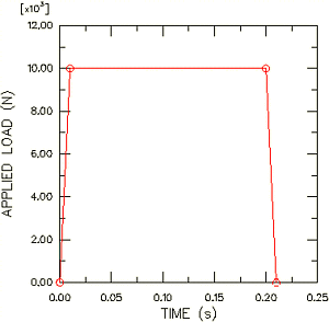
The magnitude of the applied load versus time is shown in Figure 2.

Abaqus provides scripts that replicate the complete analysis model for this problem. Run one of these scripts if you encounter difficulties following the instructions given below or if you wish to check your work. Scripts are available in the following locations:
-
A Python script for this example is provided in Cargo crane – dynamic loading. Instructions on how to fetch the script and run it within Abaqus/CAE are given in Example Files.
-
A plug-in script for this example is available in the Abaqus/CAE Plug-in toolset. To run the script from Abaqus/CAE, select ; highlight Cargo crane dynamic loading; and click . For more information about the Getting Started plug-ins, see Running the Getting Started with Abaqus examples.
Open the model database file Crane.cae, and copy the
Static model to a model named
Dynamic. The dynamic analysis model is
basically the same as the static analysis model, except for the modifications
described below.
- Material
-
In dynamic simulations the density of every material must be specified so that the mass matrix can be formed. The steel in the crane has a density of 7800 kg/m3.
In this model the material properties were specified as part of the section definition. Thus, you will need to edit the
BracingSectionandMainMemberSectionsection definitions to specify the density. In the Specify section material density field of the Edit Beam Section dialog box, enter a value of7800for each section definition.Note: If material data are defined independently of the section properties, the density is included by editing the material definition and selecting in the Edit Material dialog box. - Steps
-
The step definitions that are used for the dynamic analysis are substantially different from those used in the static analysis. Therefore, the static step created previously will be replaced by two new steps.
The first step in the dynamic analysis calculates the natural frequencies and mode shapes of the structure. The second step then uses these data to calculate the transient modal dynamic response of the cargo crane. In this analysis we will assume that everything is linear. If you want to model any nonlinearities in this simulation, direct integration of the equations of motion using the implicit dynamic procedure must be performed instead. See Nonlinear dynamics for further details.
Abaqus/Standard offers three eigenvalue extraction methods: Lanczos, automatic multi-level substructuring (AMS), and subspace iteration. Both the Lanczos and AMS methods are generally faster than subspace iteration when a large number of eigenmodes is required for a system with many degrees of freedom. While the AMS solver is more efficient for very large systems, the Lanczos solver has the most general capabilities. The subspace iteration method may be faster when only a few (less than 20) eigenmodes are needed.
We use the Lanczos eigensolver in this analysis and request 30 eigenvalues. Instead of specifying the number of modes required, it is also possible to specify the minimum and maximum frequencies of interest so that the step will complete once Abaqus/Standard has found all of the eigenvalues inside the specified range. A shift point may also be specified so that eigenvalues nearest the shift point will be extracted. By default, no minimum or maximum frequency or shift is used. If the structure is not constrained against rigid body modes, the shift value should be set to a small negative value to remove numerical problems associated with rigid body motion.
To replace the static step with a frequency extraction
step:
-
In the Model Tree, expand the Steps container. Then, click mouse button 3 on the step named Tip Load and select Replace from the menu that appears. In the Replace Step dialog box, select Frequency from the list of available Linear perturbation procedures.
Model attributes that cannot be converted will be deleted. In this case the concentrated loads are deleted because they cannot be used in a frequency extraction step. However, the boundary conditions and output requests associated with the static step are inherited by the frequency extraction step.
-
In the Basic tabbed page of the Edit Step dialog box, enter the step description
First 30
  modes
; accept the Lanczos eigensolver option; and request 30 eigenvalues. -
Rename the step to
Extract Frequenciesby clicking mouse button 3 on the nameTip Loadand selecting Rename from the menu that appears.
In structural dynamic analysis the response is usually associated with the lower modes. However, enough modes should be extracted to provide a good representation of the dynamic response of the structure. One way of checking that a sufficient number of eigenvalues has been extracted is to look at the total effective mass in each degree of freedom, which indicates how much of the mass is active in each direction of the extracted modes. The effective masses are tabulated in the data file under the eigenvalue output. Ideally, the sum of the modal effective masses for each mode in each direction should be at least 90% of the total mass. See Effect of the number of modes for more information.
The modal dynamics procedure will be used to perform the transient dynamic analysis. The transient response will be based on all the modes extracted in the first analysis step; 5% of critical damping should be used in all 30 modes.
To create a transient modal dynamics step:
-
In the Model Tree, double-click the Steps container to create a new step. Select Modal dynamics from the list of available Linear perturbation procedures, and name the step
Transient modal dynamics. Insert the step after the frequency extraction step defined above. -
In the Basic tabbed page of the Edit Step dialog box, enter the description
Crane
  Response to Dropped Load
and specify a time period of0.5and a time increment of0.005. In dynamic analysis time is a real, physical quantity. -
In the Damping tabbed page of the Edit Step dialog box, specify direct modal damping and enter a critical damping fraction of
0.05for modes1through30.
-
- Output
-
Using the Field Output Requests Manager, modify the field output requests for the
Extract
  Frequencies
step so that the Preselected defaults are selected. By default, Abaqus/Standard writes the mode shapes to the output database (.odb) file so that they can be plotted using the Visualization module. The nodal displacements for each mode shape are normalized so that the maximum displacement is unity. Thus, these results, and the corresponding stresses and strains, are not physically meaningful: they should be used only for relative comparisons.Dynamic analyses usually require many more increments than static analyses to complete. As a consequence, the volume of output from dynamic analyses can be very large, and you should control the output requests to keep the output files to a reasonable size. In this example you will request output of the deformed shape to the output database file at the end of every fifth increment. There will be 100 increments in the step (0.5/0.005); therefore, there will be 20 frames of field output.
In addition, you will write the displacements at the loaded end of the model (for example, set
Tip-a) and the reaction forces at the fixed end (setAttach) as history data to the output database file every increment so that a higher resolution of these data will be available. In dynamic analyses we are also concerned about the energy distribution in the model and what form the energy takes. Kinetic energy is present in the model as a result of the motion of the mass; strain energy is present as a result of the displacement of the structure; energy is also dissipated through damping. By default, whole model energies are written as history data to the.odbfile for the modal dynamic procedure. For this analysis you will restrict the energy output to the kinetic, internal, and viscous dissipation energies.To request output for the transient modal dynamics analysis step:
-
Open the Field Output Requests Manager. Select the cell labeled
Createdthat appears in the column labeled Transient modal dynamics (you may need to enlarge the column to see the complete step name). -
Edit the field output request so that only the nodal displacements are written to the
.odbfile every5increments. -
Open the History Output Requests Manager. Edit the default output request so that only ALLIE, ALLKE, and ALLVD are written after every increment. In addition, create two new output requests in the step labeled
Transient modal dynamics. In the first write the displacements (translations only) for the setTip-aafter every increment; in the second, the reaction forces (not the moments) for the setAttachafter every increment.
-
- Loads and boundary conditions
-
The boundary conditions are the same as for the static analysis. Since these were retained during the step replacement operation, no new boundary conditions need to be defined.
Apply a concentrated force to the tip of the crane. The magnitude of this load is time dependent, as illustrated in Figure 2. The time dependence of the load can be defined using an amplitude curve. The actual magnitude of the load applied at any point in time is obtained by multiplying the magnitude of the load (−10,000 N) by the value of the amplitude curve at that time.
To specify a time-dependent load:
-
Begin by defining an amplitude curve. In the Model Tree, double-click the Amplitudes container. Name the amplitude
Bounce, and choose the type Tabular. Enter the data shown in Table 1 in the Edit Amplitude dialog box. Accept the default selection of Step time as the time span, and specify0.25as the smoothing parameter value.Tip: Use mouse button 3 to access the table options. Table 1. Amplitude curve data. Time (sec) Amplitude 0.0 0.0 0.01 1.0 0.2 1.0 0.21 0.0 -
Now define the load. In the Model Tree, double-click the Loads container. Apply the load in the
Transient modal dynamicsstep, name the loadDyn load, and choose Concentrated force as the load type. Apply the load to setTip-b. The equation constraint defined previously between setsTip-aandTip-bmeans that the load will be carried equally by both halves of the crane. -
In the Edit Load dialog box, enter a value for CF2 of
-1.E4, and chooseBouncefor the amplitude.
In this example the structure has no initial velocities or accelerations, which is the default. However, if you wanted to define initial velocities, you could do so by selecting from the main menu bar and assigning initial translational velocities to selected regions of the model in the initial step. You would also have to edit the definition of the modal dynamics step to use initial conditions.
-
- Running the analysis
-
Create a job named
DynCranewith the following description:3-D model of light-service cargo crane dynamic analysis.Save your model in a model database file, and submit the job for analysis. Monitor the solution progress; correct any modeling errors that are detected and investigate the cause of any warning messages, taking action as necessary.