Stress linearization example | ||
| ||
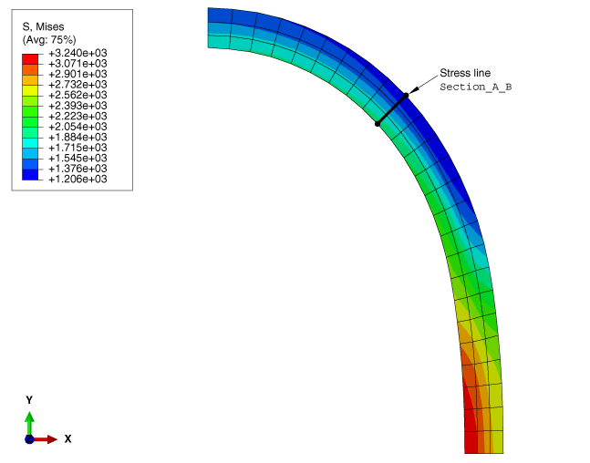
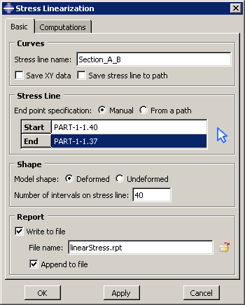
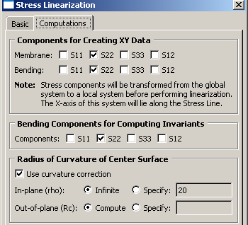
The stress line Section_A_B is defined through the vessel wall. Figure 2 and Figure 3 show the basic settings and computations, respectively, that you use to linearize the S22 stress component for the undeformed model shape.
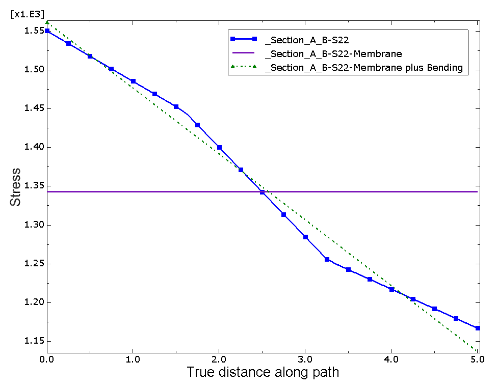
When you click or in the Stress Linearization dialog box, Abaqus/CAE creates an X–Y plot of the S22 stress component (oriented normal to the stress line) and of the resulting linearized stresses, as shown in Figure 4.
The following output is also written to a file called linearStress.rpt:
********************************************************************************
Statically Equivalent Linear Stress Distribution across a Section,
written on Thu Sep 09 11:20:19 2010

Source
-------

   ODB: Job-1.odb
   Step: Step-1
   Frame: Increment      1: Step Time =    1.000


Linearized Stresses for stress line 'Section_A_B'
  Start point, Point 1 - (18.429651260376, 26.8930339813232, 0)
  End point, Point 2   - (22.0184745788574, 30.3756923675537, 0)
  Number of intervals  - 40

------------------------------- COMPONENT RESULTS ------------------------------

                       S11         S22         S33         S12

        0            -462.376     1550.19     1450.75     74.7673
     0.125021        -453.722     1542.06     1445.35     74.6265
     0.250043        -445.068     1533.93     1439.95     74.4865
     0.375064        -436.413      1525.8     1434.55     74.3473
     0.500086        -427.759     1517.67     1429.15     74.2089
     0.625107        -419.114     1509.55     1423.76     74.0714
     0.750128         -410.46     1501.42     1418.36     73.9345
     0.87515         -401.806      1493.3     1412.96     73.7983
     1.00017         -393.152     1485.17     1407.56      73.663
     1.12519         -384.497     1477.04     1402.16     73.5284
     1.25021         -375.842     1468.92     1396.76     73.3946
     1.37524         -367.187     1460.79     1391.37     73.2615
     1.50026         -358.531     1452.67     1385.97     73.1293
     1.62528         -348.574     1443.22      1379.7     72.8307
      1.7503          -333.79     1428.85     1370.22       71.77
     1.87532         -319.007     1414.48     1360.74     70.7052
     2.00034         -304.227      1400.1     1351.26     69.6367
     2.12536         -289.448     1385.72     1341.78     68.5648
     2.25039         -274.656     1371.33     1332.29     67.4908
     2.37541         -259.847     1356.91     1322.81     66.4061
     2.50043         -245.037     1342.49     1313.32     65.3195
     2.62545         -230.228     1328.07     1303.83     64.2284
     2.75047         -215.421     1313.64     1294.34     63.1328
     2.87549         -200.613      1299.2     1284.84     62.0327
     3.00051         -185.807     1284.76     1275.34     60.9282
     3.12554         -171.002     1270.32     1265.84     59.8191
     3.25056         -156.197     1255.88     1256.34     58.7056
     3.37558         -149.216     1248.82     1251.71      57.583
      3.5006         -143.031     1242.52     1247.58     56.4609
     3.62562         -136.844     1236.21     1243.45       55.34
     3.75064         -130.658     1229.91     1239.32     54.2204
     3.87566         -124.471     1223.61     1235.19     53.1021
     4.00069         -118.283     1217.31     1231.06      51.985
     4.12571         -112.095     1211.02     1226.93     50.8691
     4.25073         -105.907     1204.72      1222.8     49.7545
     4.37575         -99.7185     1198.42     1218.67     48.6412
     4.50077         -93.5296     1192.13     1214.55      47.529
     4.62579         -87.3403     1185.83     1210.42     46.4182
     4.75081         -81.1506     1179.54      1206.3     45.3086
     4.87584         -74.9605     1173.25     1202.17     44.2002
     5.00086           -68.77     1166.96     1198.05     43.0931

     Membrane
(Average) Stress    -253.255     1342.83     1317.88     62.6971

     Bending
 Stress, Point 1     -209.122     218.613     140.324           0

  Membrane plus
Bending, Point 1    -462.376     1561.45      1458.2     62.6971

     Bending
 Stress, Point 2      184.485    -206.054    -140.324           0

  Membrane plus
Bending, Point 2      -68.77     1136.78     1177.55     62.6971

   Peak Stress,
     Point 1                0    -11.2522    -7.44933     12.0701

   Peak Stress,
     Point 2                0     30.1809     20.4932     -19.604

------------------------------- INVARIANT RESULTS -------------------------------

Bending components in equation for computing
membrane plus bending stress invariants are:   S22

                      Max.        Mid.        Min.       Tresca       Mises
                      Prin.       Prin.       Prin.      Stress      Stress
     Membrane
(Average) Stress     1345.29     1317.88    -255.714     1601.01     1587.48

  Membrane plus
Bending, Point 1     1563.61     1317.88    -255.418     1819.03     1709.46

  Membrane plus
Bending, Point 2     1317.88      1139.6    -256.077     1573.95     1492.82

   Peak Stress,
     Point 1          132.875    -10.5186    -209.855      342.73     298.128

   Peak Stress,
     Point 2          186.936     27.7292    -119.831     306.767     265.732
The S22 corresponds to the S22 stress shown in Figure 4. The actual stress values plotted in the curve Section_A_B_S22 do not appear in the report. The linearized membrane and membrane-plus-bending stress curves are generated from the values shown for S22. The reported invariants are calculated from the selected linearized components.