Large rotation of a one degree of freedom system

This problem shows an elementary example of a flexible-structure, large-rotation problem. Since it involves only one degree of freedom, it can be solved very simply in closed form. It, therefore, provides a convenient illustration of some aspects of geometrically nonlinear analysis.

This page discusses:

ProductsAbaqus/Standard

Problem description

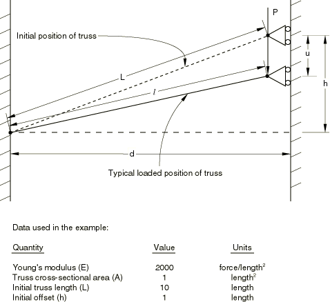
The problem is shown in Figure 1. A uniform rod, pinned at one end and free to slide in one direction at the other, is loaded so that it is initially compressed. We assume that the response of the rod is entirely linear elastic, so the only nonlinearity arises from rotation. We also assume that the initial height of the moving end of the rod above the horizontal position, h, is small compared to the horizontal distance between the supports, d, so that the strain in the rod is small so long as 0u2h.

The solution clearly involves an instability, since a nonzero force is required to begin displacing the endpoint of the rod downward, but the force must drop back to zero as the rod becomes horizontal: this horizontal position is one of unstable equilibrium. Since the problem involves only one displacement variable, no bifurcation is possible, so the behavior is quite simple compared to what can happen in systems with many degrees of freedom whose response may involve instabilities. Moreover, the displacement variable is prescribed, so there are, in fact, no unknowns in this problem. To obtain a solution at regular displacement intervals, automatic time incrementation is switched off.

The structure exhibits nonlinear response throughout its deformation, unlike typical “stiff” shell-type structures that often behave in an almost linear fashion until they buckle. Therefore, this type of problem cannot be analyzed effectively with the eigenvalue buckling procedure. However, since an exact solution to the problem is readily developed (see below), the example is a useful illustration of a simple, geometrically nonlinear analysis.

Two simple models are possible with Abaqus—one using a single truss element of type T2D2, and one using a SPRING element. There are two differences between these two models. One is the way strain is measured. Because the truss element is usually used with the standard constitutive models in Abaqus, it uses logarithmic strain. With the spring, the “strain” is calculated from the change in distance between its ends. The second difference is that the force in the truss is calculated as the stress times the area, and the area is updated as the truss deforms, using the assumption that the truss is incompressible and so has constant volume. In the spring, the force is defined immediately by the spring rate that is given in the input data times the “strain.” The exact solutions are, therefore, not the same for the two models, but they show only minor differences because the dimensions are chosen so that the strains are small throughout the deformation. The differences would be significant if large strains were involved.
Exact solution: truss model

The strain in the truss is assumed to be uniform, so the logarithmic strain definition gives

ε=ln(lL),

where l is the current length of the truss and L is its original length. From the geometry of Figure 1 we have the results

l2=d2+(h-u)2

and

L2=d2+h2,

so the strain is given in terms of the displacement as

ε=12ln(1+u(u-2h)L2),

and its first variation is

δε=1l2(u-h)δu.

We assume the material of the truss responds in a linear elastic manner, so the stress is

σ=Eε,

where E is Young's modulus. Assuming that the initial cross-sectional area is A and the material is incompressible, the virtual work statement is

LσδεAdL=Pδu.

Since the strain and stress are uniform, the integral over the volume of the truss is

LσδεAdL=ALσδε.

Introducing the above results for ε, δε, and σ, this equation gives

P=AELl2(u-h)ln(lL).

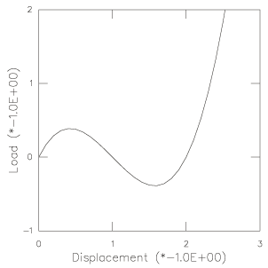
This equation is the static equilibrium equation for the system and is shown in Figure 2. largerotation1dof_truss.inp shows this problem, loaded by prescribing the displacement u throughout the step. This gives exactly the above solution.

Exact solution: spring model

The force in the spring is defined to be

F=KΔ,

where K is the spring stiffness given in the input data and Δ is the change in length of the spring. From the discussion above, we have

Δ=[d2+(h-u)2]1/2-L,

so the variation in the change in length is

δΔ=-(h-u)lδu.

The principle of virtual work gives

FδΔ=Pδu.

Using the force–relative displacement relation and the Δu relationship in this expression gives the equilibrium equation

P=-Kl(h-u){[d2+(h-u)2]1/2-L}.

largerotation1dof_spring.inp shows this version of the problem, also loaded by prescribing the displacement. This gives exactly the above response.

Results and discussion

The form of the equilibrium response is interesting because in some respects it typifies the response of some important practical cases. The initial response is stable and not very nonlinear. As the displacement increases, the system loses stiffness until a limit value of the load, Pc, is reached. The displacement at which this occurs is about 42% of h. Beyond that value the response is unstable (the system has negative stiffness) until, at a displacement of about 158% of h, it again becomes stable. (The critical displacement values and the corresponding load values can be estimated from the plot in Figure 2 or can be computed exactly from the equilibrium equations given above.) For any load in the range -Pc<P<Pc the system, thus, has three static equilibrium configurations, of which two are stable and one is unstable. Outside that range of loads the system has only one stable, static equilibrium configuration. We, thus, observe that, even in a simple elastic system with only one degree of freedom, uniqueness and stability of the solution are lost when geometric nonlinearity is introduced. In this simple case it is easy to obtain the equilibrium solution even in the unstable response phase by prescribing the only active degree of freedom of the system. In a more practical case the “Riks” algorithm must be used instead—such usage is illustrated in several other examples in this chapter.

Figures

Figure 1. Elastic, large rotation truss example.

Figure 2. Load-displacement response for truss example.