Crash simulation of a motor vehicle

This example is an elementary illustration of a motor vehicle crash simulation. The case in this example is one for which experimental results are available (Mouldenhauer, 1980), thus providing verification of the numerical results.

This page discusses:

ProductsAbaqus/Standard

Problem description

Figure 1 shows the structure, which is a scale model of a typical motor vehicle frame made of steel. The frame is moving forward at a speed of 13.89 m/s (50 km/h—about 31 miles/hour) when it collides against an oblique, rigid wall that is at 30° to its direction of motion. The objective of the analysis is to predict the history of deformation of the frame during the crash event.

The dimensions of the physical structure are shown in Figure 1. The finite element idealization is shown in Figure 2. First-order beam elements (element type B21) are used to model the frame.

The contact between the frame and a flat, rigid wall is modeled with a contact pair. The individual nodes of the frame that may be involved in contact with the wall are assigned to a node-based surface. Alternatively, the exterior surface of the frame could have been defined using an element-based surface. The rigid wall is modeled as an analytical rigid surface with a rigid body constraint in conjunction with a surface definition. The mechanical interaction between the node-based surface and the rigid surface is assumed to be frictionless.

No mesh convergence studies have been performed, but the reasonable comparison between the results of this analysis and the experimentally observed deformation suggests that the mesh is adequate, in the sense that major aspects of the behavior are predicted fairly well.

The frame is oriented along the x-axis, facing the rigid surface toward the left. The initial velocity of 13.89 m/s is prescribed for each node of the frame in the negative x-direction.

Controls and tolerances

This analysis clearly involves large deformations, so geometric nonlinearities must be included in the step definition.

The automatic time stepping algorithm for implicit dynamic integration requires that a half-increment residual tolerance be set. In an example like this we aim to obtain a solution of moderate accuracy and low computational cost. Also, this problem involves very large energy dissipation (caused by plastic deformation) and, consequently, the high frequency response will be damped rapidly. Thus, a half-increment residual tolerance that is an order of magnitude or two larger than actual typical forces should give acceptable results.

A typical force magnitude can be estimated by considering the force required to produce a fully plastic hinge in a member, based on a reasonable length of cantilever. The moment at a fully plastic hinge in a rectangular section is

M0=14h2wσ0,

where σ0 is the yield stress, h is the thickness of the section in the plane in which it bends, and w is the width of the section in the other direction. The force required to produce this moment in a cantilever of length L is

F0=M0/L.

Using the front segment of one of the side rails to compute F0 for this problem gives a value of 135 N. Based on this calculation, we set the half-increment residual tolerance to 10000 N.

Material

The material has a Young's modulus of 213 GPa and a mass density of 7850 kg/m3. It has an initial yield stress of 221.2 MPa, with isotropic hardening to a stress of 250 MPa at a plastic strain of 5.5 × 10⁻⁴ and perfect plasticity beyond that strain value.

The rigid surface is assumed to be frictionless.

Results and discussion

The implicit analysis requires about 420 increments to reach a stage in which the entire front of the frame is in contact with the rigid surface and the frame has essentially collapsed. At early stages of the analysis the time increments are very small because the initial impact initiates stress wave effects and these waves propagate throughout the model, carrying energy with them: small increments are required to model the dynamics accurately during this period. Later, the high frequency response is damped out by plastic yielding, and the time increment can be increased with no loss in accuracy.

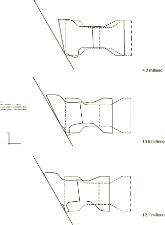
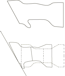
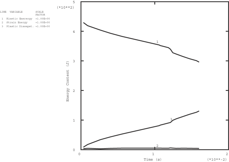
Figure 3 shows the predictions of the deformed configuration at various times and provides an illustration of the history of the event. Figure 4 compares the predicted configuration at 10 ms with the results of an experimental study. The correlation between the analysis and the experimental result is quite encouraging, especially considering the relatively coarse mesh. Figure 5 shows the variation of the total kinetic energy, strain energy, and the plastic dissipation in the frame with respect to time. After 12.5 ms about one-fifth of the initial kinetic energy has been dissipated as plastic work.

References

  1. Moldenhauer H.Oblique Impact of a Motor Vehicle (Crash simulation with Abaqus),” Control Data Corporation, Frankfurt, W. Germany, July 1980.

Figures

Figure 1. Motor vehicle frame crash study.

Figure 2. Motor vehicle frame crash study: finite element model.

Figure 3. Deformation configurations.

Figure 4. Comparison of measured and predicted configurations at 10 ms.

Figure 5. Total energy content throughout the solution.