Acoustic scattering from a rigid sphere

A rigid spherical obstacle of radius $r_0$ = 0.1 m in an unbounded acoustic medium is subjected to an incident plane wave. The analytical solution for the acoustic scattered pressure is of the form

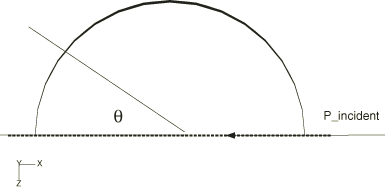
where $p_{scat}$ is the scattered acoustic pressure, $P_{incident}$ is the coefficient of the incident plane wave, $P_n\left(\cos \theta \right)$ are Legendre polynomials, $j_n\left(k{r}_0\right)$ are spherical Bessel functions of the first kind, $h_n\left(k{r}_0\right)$ are spherical Hankel functions of the first kind, $k=2\pi f/c_f$ is the acoustic wave number, $c_f=\sqrt{K_f/{\rho }_f}$ is the speed of sound, and $f$ is the frequency. The orientation is shown in Figure 1; the incident field is defined as having zero phase at the origin, which lies at the center of the sphere. The analytical solution is derived in Junger and Feit, but its complex conjugate is used for comparison to conform to the Abaqus sign convention for time-harmonic problems.

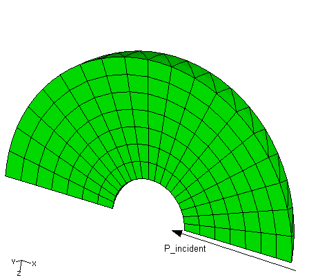
Figure 2 shows the finite element mesh using seven layers of AC3D15 elements (252 in total), with an outer radius of $r_1$ = 0.4 m and a circumferential angle of 10°. Since the problem is axisymmetric, this is sufficient to resolve the field. Planar incident wave loads of unit reference magnitude are applied to the inner surface, with the standoff point defined at the center of the sphere and the source point defined at a point along the positive x-axis. Specifying the load in this way means that Abaqus will apply loads on the surface corresponding to an incident pressure field having a value of 1 + 0 × i at the standoff point. A spherical radiation condition is imposed on the outer surface. The acoustic properties of this problem are chosen as follows: $K_f$ = 2.0736 GPa, ${\rho }_f$ = 1000 kg/m³, so that the acoustic wave speed is $c_f$ = 1440 m/s. The analysis is run using the direct-solution steady-state dynamic procedure in the range from 30 to 9000 Hertz.