Stress wave propagation illustrated | ||
| ||
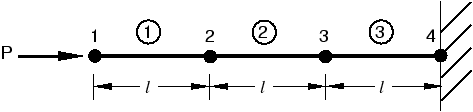
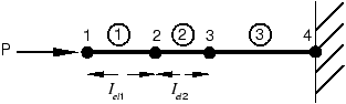
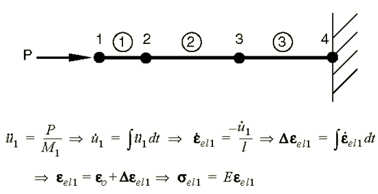
In the first time increment node 1 has an acceleration, , as a result of the concentrated force, , applied to it. The acceleration causes node 1 to have a velocity, , which, in turn, causes a strain rate, , in element 1. The increment of strain, , in element 1 is obtained by integrating the strain rate through the time of increment 1. The total strain, , is the sum of the initial strain, , and the increment in strain. In this case the initial strain is zero. Once the element strain has been calculated, the element stress, , is obtained by applying the material constitutive model. For a linear elastic material the stress is simply the elastic modulus times the total strain. This process is shown in Figure 2. Nodes 2 and 3 do not move in the first increment since no force is applied to them.
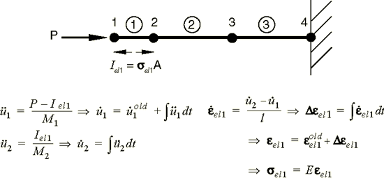
In the second increment the stresses in element 1 apply internal, element forces to the nodes associated with element 1, as shown in Figure 3. These element stresses are then used to calculate dynamic equilibrium at nodes 1 and 2.
The process continues so that at the start of the third increment there are stresses in both elements 1 and 2, and there are forces at nodes 1, 2, and 3, as shown in Figure 4. The process continues until the analysis reaches the desired total time.