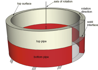
This example examines the inertia friction welding process of the pipes
shown in
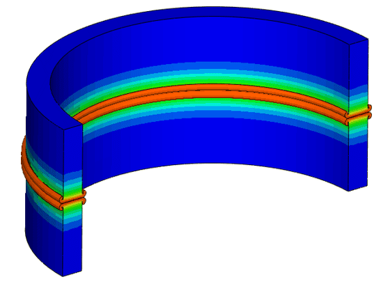
Figure 1.
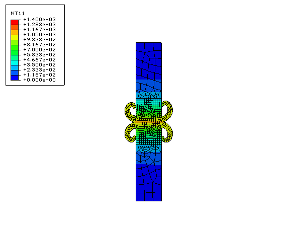
The specific arrangement considered is the resulting as-welded configuration
shown in
Figure 2.
In this weld process kinetic energy is converted rapidly to thermal energy at a
frictional interface. The resulting rapid rise in interface temperature is
exploited to produce high-quality welds. In this example the weld process is
simulated, and the initial temperature rise and material plastic flow are
observed. An important factor in the process design is control of the initial
speed of the flywheel so that, when the flywheel stops, the temperature rises
to just below the melting point, which in turn results in significant flow of
material in the region of the weld joint. Understanding the friction, material
properties, and heat transfer environment are important design aspects in an
effective inertia welding process; therefore, simulation is a helpful tool in
the process design.
Geometry
The weld process in this example is shown in
Figure 1,
where two pipes are positioned for girth-weld joining. The two pipes are
identical, each with a length of 21.0 mm, an inside radius of 42.0 mm, and an
outside radius of 48.0 mm. The pipes are adjacent, touching each other
initially at the intended weld interface.
Materials
The pipes are made of Astroloy, a high-strength alloy used in gas turbine
components.
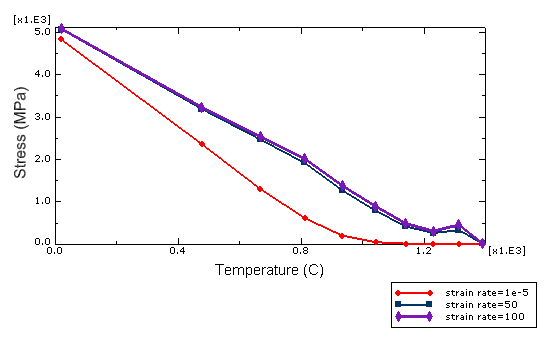
Figure 3
shows flow stress curves as a function of temperature and plastic strain rate.
At temperatures relevant to the welding process, the material is highly
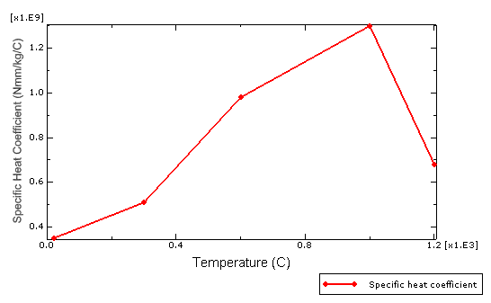
sensitive to plastic strain rate and temperature. Specific heat is a function
of temperature, as shown in
Figure 4.
Other material properties are defined as follows:
Young's modulus:
180,000 MPa
Poisson's ratio:
0.3
Density:
7.8 × 10⁻⁹ Mg/mm3
Conductivity:
14.7 W/m/°C at 20°C
28 W/m/°C at 1200°C
Initial conditions
The pipes are initially set at 20°C, representing room temperature.
Boundary conditions and loading
A pressure of 360 MPa is applied to the top surface of the upper pipe. The
initial rotational velocity of the flywheel is set at 48.17 rad/s, or 7.7
revolutions per second. The mass moment of inertia of the flywheel is 102,000
Mg mm2.
Interactions
The principal interaction occurs at the weld interface between the pipes;
however, a secondary concern is the possibility of contact of weld flash with
the side of the pipes. The weld-interface friction behavior is assumed to
follow that described by Moal and Massoni (1995), where the ratio of shear
stress to the prescribed pressure is observed to be a complex function of
interface slip rate. The heat generation from the frictional sliding, combined
with plastic deformation, contributes to the temperature rise in the pipes.
Abaqus modeling approaches and simulation techniques
Abaqus/CAE
and
Abaqus/Standard
are used together to affect the weld simulation in a way that permits extreme
deformation of the pipes in the weld region. This process is automated through
the use of Python scripts. Three cases are studied in this example.
Summary of analysis cases
Case 1
Initial flywheel velocity = 48.17 rad/s.
This case produces a successful weld.
Case 2
Initial flywheel velocity = 20.0 rad/s.
This case illustrates an unsuccessful weld scenario; the flywheel has
insufficient energy to begin the weld process.
Case 3
Initial flywheel velocity = 70.0 rad/s.
This case illustrates an unsuccessful weld scenario; the flywheel has excessive
energy, resulting in a temperature rise into the liquidus regime of the pipe
material.
The following sections discuss analysis considerations that are applicable
to all the cases. Python scripts that generate the model databases and
Abaqus/Standard
input files are provided for Case 1, with instructions in the scripts for
executing the Case 2 and Case 3 simulations.
Analysis types
The analysis is nonlinear, quasi-static with thermomechanical coupling. A
fully coupled temperature-displacement procedure is used.
Analysis techniques
The key feature required for successful simulation of this process is
remeshing. In this example, because of the large deformation near the weld
region, multiple analyses are employed to limit element distortion. These
analyses are executed in sequence, with remeshing performed between executions,
and are automated through the use of Python scripts.
At each remesh point the current model configuration represents a
significant change in the pipes' shape and in the current analysis mesh.
Abaqus/CAE
is used to extract the outer surface of the pipes, reseed the surface, and
remesh the pipe regions. This process employs the
Abaqus Scripting InterfacePartFromOdb(...)command,
which is used to extract orphan mesh parts representing the deformed pipes.
These parts are then passed to the
Part2DGeomFrom2DMesh(...)
command. This command creates a geometric Part object from
the orphan mesh imported earlier. Once the profile of the deformed part has
been created, options in the Mesh module are used to remesh the part. The new
mesh results in a new
Abaqus/Standard
analysis, and the map solution procedure maps state variables from the previous
analysis (see
Mesh-to-Mesh Solution Mapping).
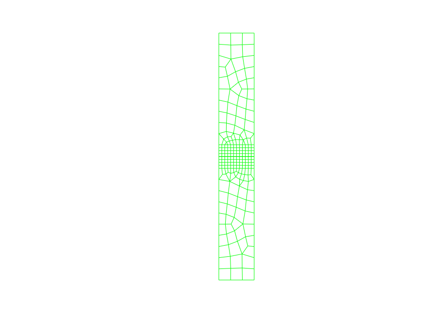
Mesh design
The pipes are modeled as axisymmetric. The element formulation used is the
fully coupled temperature-displacement axisymmetric elements with twist degrees
of freedom (element types CGAX4HT and CGAX3HT), where the twist degree of freedom enables modeling of rotation
and shear deformation in the out-of-plane direction. The hybrid formulation is
required to handle the incompressible nature of the material during the plastic
flow. The mesh is divided into two regions for each pipe. In the region near
the weld interface, smaller elements are created (see
Figure 5).
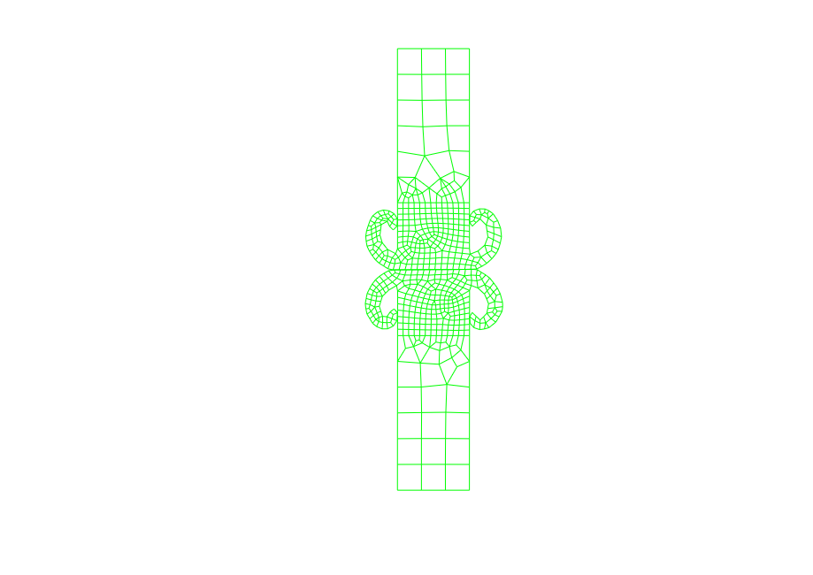
During the remeshing process, the region near the weld surface is recalculated
so that the new flash region is also meshed with smaller elements (see
Figure 6).
Materials
The material model defined for this example approximates the
high-temperature behavior of Astroloy, where it is reported by Soucail et al.
(1992) using a Norton-Hoff constitutive law to describe the temperature and
strain-rate viscoplastic behavior. A similar model is defined in
Abaqus
as a rate-dependent perfectly plastic material model. For the loading in this
model, these material parameters result in the onset of local plastic flow only
after the interface temperature has exceeded roughly 1200°C, near the material
solidus temperature of 1250°C. Above this temperature the Mises flow stress is
highly sensitive to variations in temperature and strain rate. A special
adjustment in the flow stress at high strain rates is necessary to avoid
divergence during the iteration procedure of the nonlinear solution. In the
material model definition an extreme case of stress data is defined when the
strain rate is 1.0 × 10⁶ s−1. Stress data when the strain
rate equals zero are also defined to be the same as the stress data at strain
rate 1.0 × 10⁻⁵ s−1. As a result of large deformation,
thermal expansion is not considered in the material model.
It is assumed that 90% of the inelastic deformation energy contributes to
the internal heat generation, which is the
Abaqus
default for inelastic heat fraction.
Initial conditions
An initial temperature of 20°C is specified for the entire model. The
flywheel initial velocity is specified as a solution-dependent variable initial
condition for the user element (see inertiaweld_sub.f).
Boundary conditions
The bottom pipe is fixed completely. The top pipe is free of boundary
conditions.
Loads
A pressure of 360 MPa is applied as a distributed load on the top surface of
the upper pipe.
The heat flux resulting from frictional heat generation is considered to be
many times greater than any heat lost due to convection. Thus, all boundaries
are assumed to be adiabatic.
Interactions
Five interactions are defined: four contact interactions and one
actuator-sensor interaction.
The contact interactions include a pair of interactions that define the weld interface between
the pipes, which is identified in Figure 1. This pair of interactions is symmetrical: one interaction defines the top pipe as the
main surface with the bottom pipe as the secondary surface, and the second interaction
reverses the main-secondary pairing. This “balanced main-secondary” arrangement is
important for the analysis to obtain more uniform contact pressure in the weld interface
and to avoid hourglass effects, and it is combined with a softened contact interaction
property to promote a sharing of the local contact pressure among nodes on both sides of
the interface.
To simulate the Moal and Massoni (1995) friction definition, the weld
interface friction model is defined in user subroutine
FRIC (see inertiaweld_sub.f).
This model is nonlocal in the sense that the interface pressure for all contact
nodes is the applied pressure of 360 MPa, and the sliding velocity is computed
based on the rotational angular velocity of the flywheel. This treatment of the
friction force helps stabilize the solution. Frictional heat generation is
calculated based on the frictional traction and the sliding velocity.
Nondefault contact controls definitions are used to improve convergence. These
definitions include delaying the friction computation upon contact and
automatic tolerance control to avoid contact chattering.
The two remaining contact interactions address the possibility of
self-contact near the weld area in the pipes. Self-contact in the flash area
can cause problems during remeshing: the
Part2DGeomFrom2DMesh(...)
command that was used to generate the new, current configuration geometry
performs curve-fit operations that can result in self intersections of the
boundary, which lead to invalid part topology and a meshing failure. To avoid
this problem, a softened contact model that introduces a normal pressure with a
small separation distance (−0.01 mm) is used. It is important to keep this
separation distance as small as practical to avoid causing any nonphysical
contact behavior.
The actuator-sensor interaction, which acts through user subroutine
UEL, enables the simulation of a flywheel attached to the top
pipe. The user element also has a sensor role in the analysis, measuring the
weld upset, or axial shortening, of the weld assembly. When a critical
user-defined upset distance is exceeded, the user element subroutine calls XIT to terminate the analysis and signal a remesh point. This
parameter, the allowed “upset distance,” correlates well with the extent of
mesh deformation in the weld region.
Analysis steps
Each of the analyses run in the simulation sequence uses a single fully
coupled temperature-displacement step. Since the duration of the step is
controlled by the user element, as described above, it is not known a priori
for each analysis. Therefore, the step duration is set in each analysis to be
the total remaining time for the simulation, a time that is reached only in the
final analysis in the simulation sequence.
Solution controls
Full Newton iteration is used for the nonlinear solution. Automatic time
stepping is based on the maximum temperature change in each increment. Results
from the previous increment are used as the initial guess in the current
increment, with the parabolic extrapolation technique adopted to transfer the
previous state to the current state.
Heat fluxes due to frictional heat generation can cause contact chattering.
To overcome this difficulty, contact controls with the automatic tolerances
parameter are used.
Output requests
Field output of temperature, stress, and equivalent plastic strain is
requested. Various energy measures are requested for history output, allowing
you to record the flywheel energy change during the simulation.
Convergence
In general, convergence is difficult in the initial increments, especially
after remeshing. More iterations are also observed near the end of the
analysis-run sequence when deformation increases and the mesh distortion
becomes severe.
Run procedure
This example is run using the
Abaqus/CAE
Python scripts provided. Use the following command to run the example:
abaqus cae –script inertiaweld.py
The simulation results in a sequence of separate output database
(.odb) files, each corresponding to one of the analyses.
For postprocessing convenience a number of scripts are provided for
evaluating simulation results across the sequence of files. Use the following
command to create the inertia_weld_animation.avi animation
file:
abaqus cae –script inertiaweld_movie.py
Run the following Python scripts to create X–Y
plots:
This example focuses mainly on the successful weld case, Case 1. Case 2 and
Case 3 are provided to show the precarious nature of the inertia weld process,
where it is essential to select the flywheel size correctly, measured by the
mass moment of inertia, and the initial velocity of the flywheel. Case 2 and
Case 3 illustrate why simulation is a valuable tool in the weld process design
as each case clearly shows that the selected process parameters do not result
in a successful weld.
Welding success: Case 1
The example simulation creates multiple output database
(.odb) files, requiring 22 remeshings to reach the
simulation time of 5.0 seconds. The results in the first analysis before the
first remeshing show that the temperature rises very fast near the weld
interface. At about 1.6 seconds the temperature reaches 1172°C and the material
starts to flow, squeezing out to form flash (see
Figure 7).
After 2.31 seconds and 5 remeshings the flash extends enough to fold back and
contact the pipe (see
Figure 8).
At 3.51 seconds the flywheel velocity slows down to 3.51 rad/s, the temperature
starts to drop, and the material flow slows down. At this point a considerable
amount of flash build-up can be observed (see
Figure 9).
After 5.0 seconds the flywheel stops, the temperature drops below 1000°C, and
the pipes are welded (see
Figure 10).
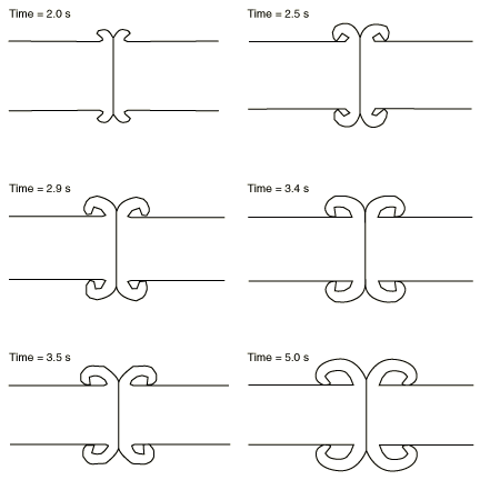
The flash prediction in
Figure 11
is in good agreement with those shown by Moal and Massoni (1995).
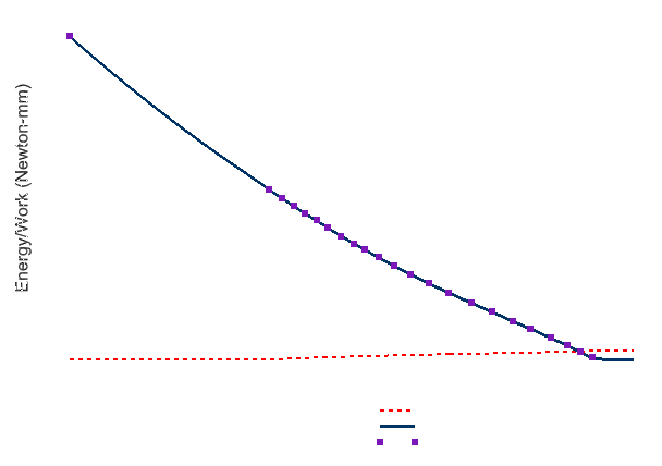
Figure 12
plots the kinetic energy history (created with inertiaweld_xy.py)
and shows how the flywheel slows down and stops. The “RemeshPoints” marks
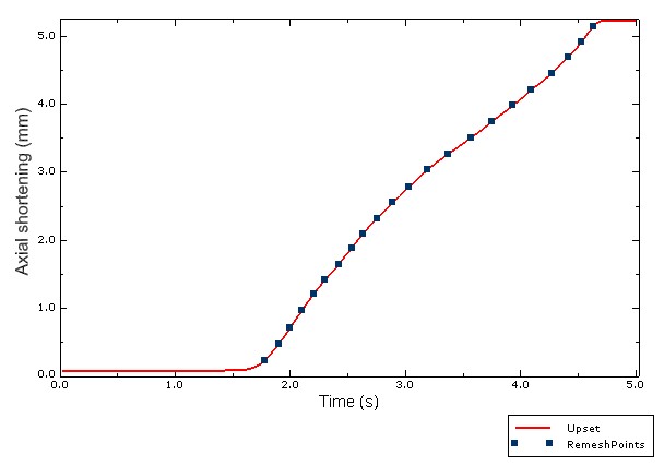
indicate the time at which the remeshing procedure occurred. The upset distance
during the welding process is shown in
Figure 13
(created with inertiaweld_upset.py).
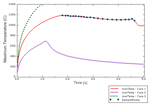
The curve of the maximum temperature for Case 1 is plotted in
Figure 14
(created with inertiaweld_maxtemp.py).
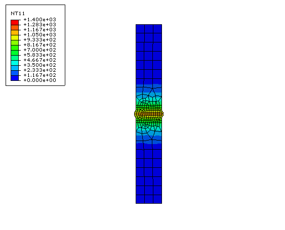
Insufficient flywheel energy: Case 2
If a lower initial flywheel velocity is selected, the temperature may not
reach a level high enough for the material to flow. For this case the initial
velocity is reduced to 20 rad/s.
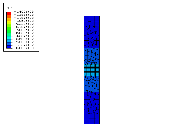
Figure 15
shows the configuration at 5.0 seconds, where not much deformation is observed
and the temperature near the interface is about 250°C. The history plot of the
maximum temperature for Case 2 in
Figure 14
shows the pipe temperature reaches only 700°C about 1.1 seconds before it cools
down. In this case the material is not hot enough to initiate the material
flow, and welding will not be successful.
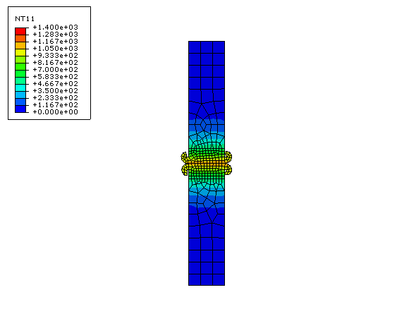
Excessive flywheel energy: Case 3
If a higher initial velocity of the flywheel is selected, the material
becomes so hot that it starts to melt. For this case the initial velocity of
the flywheel is set at 70 rad/s.
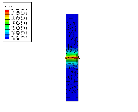
Figure 16
shows that the temperature rapidly reaches 1360°C (at about 0.9 seconds), which
is well beyond the melting temperature at 1250°C, before convergence failures
stop the analysis.
Figure 14
shows the history plot of the maximum temperature in the pipes for Case 3. In
this case the excessive energy results in melting and a failed weld.
Fortran file containing user subroutines
UEL and
FRIC.
References
Moal, A., and E.
Massoni, “Finite Element Simulation of the Inertia
Welding of Two Similar Parts,” Engineering Computations, vol.
12, pp. 497–512, 1995.
Soucail, M., A.
Moal, L. Naze, E.
Massoni, C. Levaillant, and
Y. Bienvenu,
“Microstructural Study and
Numerical Simulation of Inertia Friction Welding of Astroloy,”
7th International Symposium on Superalloys, Seven Springs, USA, 1992.
Figures
Figure 1. Inertia weld configuration for two pipes. Figure 2. Half-section view of the inertia welding final as-welded configuration
showing the temperature fields at 5 seconds after welding begins. Figure 3. Flow stress curves. Figure 4. Specific heat curve (N mm/kg/°C). Figure 5. Initial mesh. Figure 6. Typical mesh design on a deformed configuration pair of parts. Figure 7. Temperature at 1.78 sec. Figure 8. Temperature at 2.31 sec. Figure 9. Temperature at 3.51 sec. Figure 10. Temperature at 5.0 sec. Figure 11. Flash prediction in current analysis. Figure 12. Kinetic energy history showing the flywheel slowdown. Figure 13. Assembly upset (shortening) history. Figure 14. Maximum temperature history comparisons of the three cases. Case 1:
Successful weld; Case 2: Failed weld with insufficient flywheel energy; Case 3:
Failed weld with excessive flywheel energy. Figure 15. Temperature distribution at 5.0 sec for Case 2 (insufficient flywheel
energy for welding). Figure 16. Temperature distribution at 0.9 sec for Case 3 (excessive initial
flywheel energy results in a rapid temperature rise into the melting
regime).