This example shows the geometric collapse study of a stiff,
shell-type structure using
Abaqus.
The problem is that of a square, thin, elastic plate, simply
supported on all four edges and compressed in one direction (see
Figure 1).
The analytical solution for the buckling load for this case (see Timoshenko
and Gere, 1961, Section 9.2) is
Ncrit=4π2Db2,
where Ncrit
is the critical value of the edge load per unit length of the edge,
b is the length of each edge of the plate, and
D=Et3/12(1-ν2)
is the elastic bending stiffness of the plate, with Young's modulus
E, Poisson's ratio ν,
and plate thickness t.
The corresponding buckling mode is a transverse displacement of
w=Acosπxbcosπyb
in the coordinate system of
Figure 1.
Here A is an arbitrary magnitude.
Problem description
No particular units are used in this example; the values chosen are taken to
be in a consistent set. The length of the edge of the square plate is 2 and the
thickness is 0.01, so the plate is rather thin (L/t=
200). Since the solution is known to be symmetric, only one-quarter of the
plate is modeled. Meshes of 2 × 2 or 4 × 4 elements are used. Since the form of
the prebuckled and postbuckled solutions is rather smooth in this case, even
these relatively coarse meshes should give reasonably accurate results for the
buckling load.
The material is assumed to be isotropic elastic, with a Young's modulus of
108 and a Poisson's ratio of 0.3.
The boundary conditions on the model are
Symmetry about x=0.
This requires ux=ϕy=ϕz=0
on that edge of the mesh.
Symmetry about y=0.
This requires uy=ϕx=ϕz=0
on that edge of the mesh.
Simple support on the edge at x=b/2.
This requires uz=ϕx=
0 on that edge of the mesh.
Simple support on the edge at y=b/2.
This requires uz=ϕy=0
on that edge of the mesh.
Loading
Two versions of the problem are used: one in which the plate is loaded in
one direction by uniform edge loads, and one in which the plate is compressed
by raising its temperature with the plate constrained in one direction against
overall thermal expansion.
For the mechanically loaded case the edge loads are given as point loads on
the edge nodes. Since the second-order elements (S8R5, S9R5, STRI65) use quadratic interpolation along their edges, consistent
distribution of a uniform load gives equivalent point loads in the ratio 1:4:1
at the corner, midside, and corner nodes, respectively (Simpson's integration
rule). The first-order elements (S4R5, S4R, S3R, STRI3) are based on linear in-plane displacements so that the uniform
edge loading gives equal point loads at the nodes on the edge.
Eigenvalue buckling prediction
Stiff shell collapse studies are typically begun with eigenvalue buckling
estimates. Such estimates are usually accurate in cases of stiff shells—that
is, when the prebuckle response is essentially linear; when the collapse is not
catastrophic, so the structure is not excessively sensitive to imperfections;
and when the response is elastic. As will be seen later, these conditions are
fulfilled by this example.
Eigenvalue buckling estimates are obtained by using the eigenvalue buckling
procedure (Eigenvalue Buckling Prediction).
Since the eigenvalue buckling procedure is a linear perturbation procedure the
size of the load is immaterial because the response is proportional to the
magnitude of the load.
Abaqus
will predict the buckling modes and corresponding eigenvalues. In this case
three modes are requested. The lowest buckling load estimates are shown in
Table 1.
All of the meshes except the 4 × 4 mesh of element type S3R give reasonable predictions. The S3R elements give a higher estimate of lowest buckling load because
the constant bending strain approximation results in a stiffer response. The
most accurate results are those provided by element types S8R5 and S9R5.
Load-displacement studies on imperfect geometries
The next phase of a typical collapse analysis is to perform a
load-displacement analysis to ensure that the eigenvalue buckling prediction
already obtained is accurate and, at the same time, to investigate the effect
of initial geometric imperfection on the load-displacement response. In this
way concerns about imperfection sensitivity (unstable postbuckling response)
can be addressed. The eigenvalue analysis is useful in providing guidance about
mesh design for these more expensive load-displacement studies: mesh
convergence studies can be performed as part of the eigenvalue analysis, which
is usually significantly less expensive than the load-deflection analysis.
For the load-displacement analysis the perfect geometry must be “seeded”
with an imperfection to cause it to collapse. It is possible that a problem run
with perfect geometry may never buckle numerically at reasonable load levels
because the model has absolutely no prebuckled displacement in the postbuckled
mode and, thus, no ability to switch to that mode. Presumably an imperfection
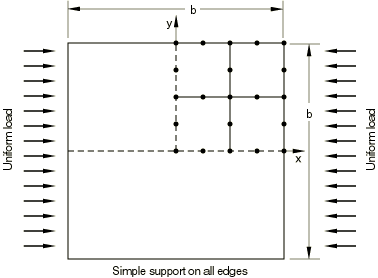
in the form of the buckling mode would be the most critical. In this example,
for simplicity, we use instead a bilinear imperfection:
z(x,y)=AI(1-2xb)(1-2yb).
So long as the imperfection contains the mode into which the structure
wishes to collapse, it is presumed that any imperfection will provide the
necessary perturbation of the solution.
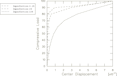
The imperfection magnitude, AI,
is taken as 0.1%, 1%, and 10% of the plate thickness. Since we expect a buckle
at a load of about 90.4, the edge load is applied by requesting that the load
be increased monotonically up to a value of 100, starting with an increment of
10. Normally the Riks method would be chosen if the postbuckling response is
unstable. It is not necessary for this case.
In all cases where a sudden loss of stiffness is expected (as here, when the
imperfection is very small) it is essential that equilibrium be satisfied
closely; otherwise it is possible for the solution to fail to switch to the
alternate branch of the solution. The default equilibrium tolerances used in
Abaqus
are rather tight by engineering standards, as experience shows that less
demanding equilibrium control may fail to pick up the buckle in the case of
almost perfect geometry.
Results and discussion
The numerical results for the mechanically loaded case are summarized in
Figure 2,
where the displacement of the center point of the plate is plotted as a
function of compressive force. The case with the smallest imperfection (0.1% of
the thickness) shows a very sharp loss of stiffness at an applied load of about
90. This is essentially the eigenvalue solution (90.4). As the initial
imperfection magnitude is increased, the behavior becomes smoother, as would be
expected. The plate shows positive stiffness up to the maximum loading applied,
even when the imperfection is very small. Thus, in this case the buckling is
not an unstable failure; the plate is, therefore, not very sensitive to
imperfection. In cases of unstable postbuckling response it is usually easiest
to approach the analysis by studying the larger imperfection magnitudes first,
since then the response is smoothest.
The stress just at buckling with the smallest imperfection is about 9000. An
interesting alternative case is where the edges parallel to the
y-axis are restrained in the
x-direction (that is, ux=ϕz=0),
and the temperature of the plate is raised. This should give the same
prebuckled stress field in the plate; and, thus, critical temperature changes
should be those that give the same critical stress. To investigate this case,
we use a thermal expansion coefficient of 10−6 (strain per unit
temperature rise) so that in the prebuckled state the critical stress should
occur at a temperature of 90°. The results of such a thermally loaded case for
the smallest imperfection studied are shown in
Figure 3.
The behaviors of the mechanically loaded case and the thermally loaded case are
quite similar, with the thermally loaded case showing rather less displacement
after buckling. This is to be expected, since thermal loading causes strain,
whereas mechanical loading requires a specific stress state to retain
equilibrium.
The same thermally loaded case is solved using the Riks approach to verify
the
Abaqus
capability for using the Riks algorithm with thermal loading only. The
temperature-displacement curves for the incremental static analysis versus the
Riks analysis are very similar, with the smoother curve obtained by the Riks
approach for strain levels between 0.5 × 10⁻³ and 2 ×
10−3. The Riks algorithm chooses smaller temperature increments,
thus requiring more increments to apply the same total temperature rise.