Use
Abaqus/CAE
to create a three-dimensional model of the stiffened plate.
Abaqus
provides scripts that replicate the complete analysis model for this problem.
Run one of these scripts if you encounter difficulties following the
instructions given below or if you wish to check your work. Scripts are
available in the following locations:
A plug-in script for this example is available in the
Abaqus/CAE
Plug-in toolset. To run the script from
Abaqus/CAE,
select Plug-insAbaqusGetting
Started; highlight Blast loading on a
stiffened plate; and click Run. For more
information about the Getting Started plug-ins, see
Running the Getting Started with Abaqus examples.
Defining the model
geometry
Create a three-dimensional, deformable part with an extruded shell base
feature to represent the plate. Use an approximate part size of
5.0, and name the part
Plate. A suggested approach for creating the
part geometry shown in
Figure 1
is summarized in the following procedure:
Figure 1. Sketch of the stiffened plate (with grid spacing doubled).
To create the stiffened plate geometry:
To define the plate geometry, use the Create Lines:
Connected tool to sketch an arbitrary horizontal line.
To define the stiffener geometry, add three vertical lines extending up from
the plate. The horizontal position of these lines is arbitrary at this stage,
but their endpoints must snap to the horizontal line.
Constrain the three vertical lines so they are of equal length, and
dimension one of them so that it is 0.1 m long.
Split the plate at the points where it intersects the stiffeners.
Apply horizontal constraints to each of the horizontal segments of the line.
Apply equal length constraints to the four horizontal segments of the line.
Dimension the horizontal distance between the plate endpoints, and set the
value to 2.0 m.
Extrude the sketch to a depth of 2.0 m to create the plate.
Defining the material properties
Define the material and section properties for the plate and the stiffeners.
Create a material named Steel with a mass
density of 7800 kg/m3, a Young's
modulus of 210.0E9 Pa, and a Poisson's ratio of
0.3. At this stage we do not know whether there
will be any plastic deformation, but we know the value of the yield stress and
the details of the post-yield behavior for this steel. We will include this
information in the material definition. The initial yield stress is 300 MPa,
and the yield stress increases to 400 MPa at a plastic strain of 35%. To define
the plastic material properties, enter the yield stress and plastic strain data
shown in
Figure 1.
The plasticity stress-strain curve is shown in
Figure 2.
Figure 2. Yield stress versus plastic strain.
During the analysis
Abaqus
calculates values of yield stress from the current values of plastic strain. As
discussed earlier, the process of lookup and interpolation is most efficient
when the stress-strain data are at equally spaced values of plastic strain. To
avoid having the user input regular data,
Abaqus/Explicit
automatically regularizes the data. In this case the data are regularized by
Abaqus/Explicit
by expanding the data to 15 equally spaced points with increments of 0.025.
To illustrate the error message that is produced when
Abaqus/Explicit
cannot regularize the material data, you could set the regularization tolerance
to 0.001 (in the Edit Material dialog box, select
GeneralRegularization)
and include one additional data pair, as shown in
Table 1.
You can add a row by clicking mouse button 3 in the table and selecting
Insert Row from the menu that appears.
Table 1. Modified plasticity data.
Yield Stress (Pa)
Plastic Strain
300.0E6
0.000
349.0E6
0.001
350.0E6
0.025
375.0E6
0.100
394.0E6
0.200
400.0E6
0.350
The combination of the low tolerance value and the small interval in the
user-defined data would lead to difficulty in regularizing this material
definition. The following error message would be written to the status
(.sta) file and displayed in the Job
Monitor dialog box in the
Job module:
***ERROR: Failed to regularize material data for material STEEL. Please check your input data to see if they meet both criteria as explained in "MATERIAL DATA DEFINITION" section of the Abaqus Materials Guide. In general, regularization is more difficult if the smallest interval defined by the user is small compared to the range of the independent variable.
Before continuing, set the regularization tolerance back to the default
value (0.03) and remove the additional pair of data points.
Creating and
assigning section properties
Create two homogeneous shell section properties, each referring to the steel
material definition but specifying different shell thicknesses. Name the first
shell section property PlateSection, select
Steel as the material, and specify
0.025 m as the value for the Shell
thickness. Name the second shell section property
StiffSection, select
Steel as the material, and specify
0.0125 m as the value for the Shell
thickness.
Assign the StiffSection definition to the
stiffeners (use
ShiftClick to
select multiple regions in the viewport).
Before assigning the PlateSection
definition to the plate, consider the following. If the plate and the
stiffeners are joined directly at their midsurfaces (this is the default
behavior), an area of material overlap will occur, as shown in
Figure 3.
Figure 3. Overlapping material.
Although the thicknesses of the plate and stiffener are small in comparison
to the overall dimensions of the structure (so that this overlapping material
and the extra stiffness it creates would have little effect on the analysis
results), a more precise model can be created by offsetting the plate reference
surface from its midsurface. This technique allows the stiffeners to butt up
against the plate without overlapping any material with the plate, as shown in
Figure 4.
Figure 4. Stiffener joint in which the plate's reference surface is offset from
its midsurface.
To determine whether to offset the plate reference surface to its positive
(SPOS) or negative
(SNEG) side, query the shell normals
(ToolsQuery)
and note the color of the side of the plate facing the stiffeners (brown is the
positive side; purple is the negative side). If necessary, flip the plate
normals (AssignElement
Normal) so that its segments have consistent
normals. Then assign the PlateSection
definition to the regions of the plate. In the Edit Section
Assignment dialog box, set the shell offset to Top
surface if the brown (positive) side of the plate faces the
stiffeners and Bottom surface if the purple (negative)
side faces the stiffeners.
To verify the offset, select
ViewPart Display
Options. In the Part Display
Options dialog box that appears, toggle on Render shell
thickness. If necessary, modify the offset to remove any overlap.
The model can be color-coded according to section assignment to verify that
properties were assigned correctly (select Sections from
the Color Code toolbar).
Creating an
assembly
Create a dependent instance of the plate. Use the default rectangular
coordinate system, with the plate lying in the 1–3 plane.
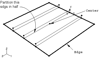
At this point, it is convenient to create the geometry sets that will be
used to specify boundary conditions and output requests. Create an
assembly-level set named Edge for the plate
edges and another named Center at the center of
the intersection of the plate and the middle stiffener, as shown in
Figure 5.
To create the set Center, you need to first
partition the edge of the original part in half using the Partition
Edge: Enter Parameter
tool (the partition must be created in either the Part or Property
module since this is a dependent part instance).
Figure 5. Geometry sets.
Defining steps
and output requests
Create a single dynamic, explicit step. Name the step
Blast, and specify the following step
description: Apply blast loading. Enter a
value of 50E-3 s for the time period of the
step.
In general, you should try to limit the number of frames written during the
analysis to keep the size of the output database file reasonable. In this
analysis saving information every 2 ms should provide sufficient detail to
study the response of the structure. Edit the default output request
F-Output-1, and set the number of intervals
during the step at which preselected field data are saved to 25. This ensures
that the selected data are written every 2 ms since the total time for the step
is 50 ms.
A more detailed set of output for selected regions of the model can be saved
as history output. Create a history output request named
Center-U2 for the step
Blast. Select
Center as the output domain, and select
U2 as the translation output variable. Enter
500 as the number of intervals at which the
output will be saved during the analysis.
Prescribing
boundary conditions and loads
Next, define the boundary conditions used in this analysis. In the step
Blast, create a
Symmetry/Antisymmetry/Encastre
mechanical boundary condition named Fix edges.
Apply the boundary condition to the edges of the plate using the geometry set
Edge, and specify ENCASTRE (U1 = U2
= U3 = UR1 = UR2 = UR3 = 0) to fully constrain the set.
The plate will be subjected to a load that varies with time: the pressure
increases rapidly from zero at the start of the analysis to its maximum of 7.0
× 105 Pa in 1 ms, at which point it remains constant for 9 ms before
dropping back to zero in another 10 ms. It then remains at zero for the
remainder of the analysis. See
Figure 6
for details.
Figure 6. Pressure load as a function of time.
Define a tabular amplitude curve named Blast.
Enter the amplitude data given in
Table 2,
and specify a smoothing parameter of 0.0.
Table 2. Blast load amplitude.
Time
Amplitude
0.0
0.0
1.0E−3
7.0E5
10.0E−3
7.0E5
20.0E−3
0.0
50.0E−3
0.0
Next, define the pressure loading. Since the magnitude of the load will be
defined by the amplitude definition, you need to apply only a unit pressure to
the plate. Apply the pressure so that it pushes against the top of the plate
(where the stiffeners are on the bottom of the plate). Such a pressure load
will place the outer fibers of the stiffeners in tension.
To define the pressure loading:
In the
Model Tree,
double-click the Loads container. In the Create
Load dialog box that appears, name the load Pressure
load and select Blast as the
step in which it will be applied. Select Mechanical as the
load category and Pressure as the load type. Click
Continue.
Select all the surfaces associated with the plate. When the appropriate
surfaces are selected, click Done.
Abaqus/CAE
uses two different colors to indicate the two sides of the shell surface. To
complete the load definition, the colors must be consistent on each side of the
plate.
If necessary, select Flip a surface in the prompt
area to flip the colors for a region of the plate. Repeat this procedure until
all of the faces on the top of the plate are the same color.
In the prompt area, select the color representing the side of the plate
without the stiffeners.
In the Edit Load dialog box that appears, specify a
uniform pressure of 1.0 Pa, and select the
amplitude definition Blast. Click
OK to complete the load definition.
The plate load and boundary conditions are shown in
Figure 7.
Figure 7. Pressure load and boundary conditions.
Creating the
mesh and defining a job
Seed the part with a global element size of
0.1. In addition, select
SeedEdges
and specify that two elements be created along the height of each stiffener (in
the Local Seeds dialog box, select By
number as the method and set the number of elements to
2; toggle on the option to create a set
containing the selected edges). Mesh the plate and stiffeners using
quadrilateral shell elements (S4R) from the Explicit element library. The
resulting mesh is shown in
Figure 8.
This relatively coarse mesh provides moderate accuracy while keeping the
solution time to a minimum.
Figure 8. Meshed plate.
Create a job named BlastLoad. Specify the
following job description: Blast load on a flat plate with
stiffeners: S4R elements (20x20 mesh) Normal stiffeners
(20x2).
Save your model in a model database file, and submit the job for analysis.
Monitor the solution progress; correct any modeling errors that are detected,
and investigate the cause of any warning messages.


 tool (the partition must be created in either the Part or Property
module since this is a dependent part instance).
tool (the partition must be created in either the Part or Property
module since this is a dependent part instance).