Aeroelastic Supersonic Flow over Long, Thin-Walled Cylinders

This is a more complex example illustrating how to embed the SIMULIA Co-Simulation Services API in a client that computes pressures associated with hypersonic flow on cylindrical panels.

This page discusses:

This example studies the flutter behavior of infinitely long thin-walled cylinder subjected to aero-elastic supersonic flow. Such simulations are important to understand the complex nonlinear behavior that is present in high-speed flight vehicles such as aircraft, rockets, and launch vehicles, where one side of the structure is exposed to supersonic flow and the other side to still air.

Problem Description

The supersonic flow is computed using the Third-order Piston Theory. Third-order Piston Theory is a popular modeling technique used for supersonic and hypersonic aero-elastic analysis. We provide a standalone program, thirdOrderPiston, that computes the pressure as a function of the time and deformation computed by Abaqus/Explicit. We compare the results to analytical derived results from L. Librescu, et. al. (2002).

The structure consists of an aluminum cylindrical panel with a curvature 0.1 m and a thickness of 0.01 m. The finite element model consists of a symmetric section with an arc length of 1 m. The material properties for the panels are as follows:

Young's modulus 7 × 10¹⁰ N/m2
Poisson's ratio 0.3
Density 3000 kg/m3

The third-order piston program uses the following fluid properties to model air:

Isentropic gas coefficient 1.4
Speed of sound 340.3 m/s
Density 1.225 kg/m3

We assume an absolute pressure of 101328 N/m2 . You can vary the speed by changing the variable, M_INF, in the third-order piston program.

The mesh used by the third-order piston program is generated and can be varied by modifying the variables myModel->numElemsMesh and myModel->numLayerMesh in the program. The upper and lower edges of the panel are pinned. Due to symmetry, the displacements in the axial directions are fixed.

Figure 1 shows the Abaqus mesh. There are 40 S4R elements in the circumferential direction.
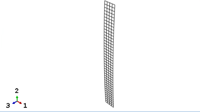
Figure 1. Abaqus mesh of the panel segment.

You could have used one layer of elements in the cylindrical direction with a symmetry boundary condition; however, we use four layers of elements to illustrate mapping.

The upper and lower edges of the panel are pinned. Due to symmetry, the displacements in the axial directions are fixed. To get an initial nonzero pressure field, we introduce an initial imperfection in the first analysis step by applying a single load at the panel center. In the second step, we import the pressure computed by the third-order piston program.

Since Abaqus/Explicit cannot import pressure loads directly, we convert the pressure into a traction vector. The mapper then integrates the traction to concentrated force for Abaqus/Explicit.
Third-Order Piston Theory

The pressure field is computed according to third-order piston theory

p − p ∞ = − k p ∞ M ∞ [ A + M ∞ 1 + k 4 A 2 + M ∞ 2 1 + k 12 A 3 ] ,
where
A = 1 M ∞ a ∞ ∂ w ∂ t + ∂ w ∂ ξ ,
and p ∞ is the free stream pressure of the undisturbed flow (Pa), k is the isentropic gas coefficient, and M ∞ is the undisturbed flight Mach number.

The spatial derivative is approximated by the central difference method:

∂ w ∂ ξ = w c e n t e r + 1 / 2 − w c e n t e r − 1 / 2 l ,
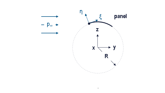
where w is the transverse displacement, and l is the element edge length in the ξ -direction shown in Figure 2.

Figure 2. Modeling schematic.

Compiling the Third-Order Piston Simulator

If you have not already done so, extract the SIMULIA Co-Simulation Services API kit as described in Extracting the SIMULIA Co-Simulation Services API Kit. For information about compiling your client, see Compiling your Application with SIMULIA Co-Simulation Services. Typical compile options for the client are as follows:

On Windows:

cl /c /W0 /MD /TP /I<location of CSS header files> thirdOrderPiston.cpp

On Linux:

g++ -c -fPIC -w -Wno-deprecated -I <location of CSS header files> thirdOrderPiston.cpp

Linking the Third-Order Piston Simulator

Depending on how you load the dynamic libraries, the linker might need access to the SIMULIA Co-Simulation Services dynamic libraries. For information about linking your client, see Linking the SIMULIA Co-Simulation Services to Your Application. Typical link options for the client are as follows:

On Windows:

link /nologo /INCREMENTAL:NO /subsystem:console /machine:AMD64 /STACK:20000000 /NODEFAULTLIB:LIBC.LIB /DEFAULTLIB:kernel32.lib /DEFAULTLIB:user32.lib /DEFAULTLIB:advapi32.lib /FIXED:NO /LARGEADDRESSAWARE /out:.\thirdOrderPiston.exe .\thirdOrderPiston.obj /LIBPATH:<location of CSS .dll> ABQSMACseModules.lib msvcrt.lib

On Linux:

g++ -fPIC -Wl,-Bdynamic -Wl,--add-needed -o thirdOrderPiston ./thirdOrderPiston.o -L<path to CSS .so> -lABQSMACseModules

Running the Coupled Simulation

You run three processes for the coupled simulation:

  • the SIMULIA Co-Simulation Services Director;
  • the third-order piston simulator that computes the pressure; and
  • Abaqus/Explicit analysis.
We recommend that you run these in three separate command shells so that you can monitor each process during the development and debugging stages.

The SIMULIA Co-Simulation Services Director process and its command line arguments are described in SIMULIA Co-Simulation Services Director. You can start the SIMULIA Co-Simulation Services Director process by starting the SMACseCtlMain.exe function or by using the abaqus cse execution procedure.

The third-order piston simulator's command line arguments are as follows:

csedirector
Director in charge of the coupled simulation.

Specify the host:port where host is the name of the machine where the SIMULIA Co-Simulation Services Director port is launched, and port is the listener port used by the SIMULIA Co-Simulation Services Director.

speed
Mach number for the undisturbed speed.

Use the commands below to start the coupled simulation. The SIMULIA Co-Simulation Services Director is launched on host mars with listener port 92000.

abaqus -cse -config thirdOrderPiston_xpl_config.xml -listenerport 92000
thirdOrderPiston -speed 4.16 -csedirector mars:92000
abaqus -job thirdOrderPiston_xpl -double_both -csedirector mars:92000

Results

The co-simulation computes the Mach flutter of MFnumerical ≈ 4.17. The numerical solution matches the analytical expectations according to L. Librescu, et. al. (2002) within less than one percent.

To determine the numerical Mach flutter, MFnumerical, we plot the displacements in the global z-direction of the center node of the panel. Figure 3 shows a stable behavior of the panel for a Mach number of M∞ = 4.16.

Figure 3. Center node displacement for M∞ = 4.16.

On the contrary, the displacements for a Mach number of M∞ = 4.18 (shown in Figure 4) do not damp out, which indicates that the numerical computed flutter speed is MFnumerical ≈ 4.17.
Figure 4. Center node displacement for M∞ = 4.18.

Files

The C++ code for the Third-order Piston Theory, the Abaqus input file, and the configuration files are available in the examples/ folder in the SIMULIA Co-Simulation Services API kit. If you have Abaqus installed, you can also use the abaqus fetch execution procedure .

thirdOrderPiston.cpp
C++ code for third-order piston program.
thirdOrderPiston_xpl.inp
Abaqus/Explicit input file for third-order piston model.
thirdOrderPiston_xpl_config.xml
Configuration file for third-order piston example.

References

  1. Librescu,  L.,  P. Marzocca, and W. A. Silva, “Supersonic/Hypersonic Flutter and Postflutter of Geometrically Imperfect Circular Cylindrical Panels,” Journal of Spacecraft and Rockets, vol. 39, no. 5, 2002.