Dual Mass-Spring Systems

This example illustrates how to embed the SIMULIA Co-Simulation Services API in a simple client that computes the dynamic response of a coupled dual mass-spring system.

The dual mass-spring example serves as a good starting point.

You learn how to:

  • Embed the SIMULIA Co-Simulation Services API into a client.
  • Compile and link the SIMULIA Co-Simulation Services to the client.
  • Run a co-simulation between two mass-spring clients.
  • Run a co-simulation between a mass-spring client and Abaqus/Standard.
  • Author the Co-Simulation Configuration file for the advanced iterative coupling schemes.

This page discusses:

This example is designed to illustrate stability issues associated with the segregated solution approach. We encourage you to experiment by changing the stiffness and mass distribution ratios between the subsystems, coupling step sizes, and coupling algorithms.

Problem Description

Figure 1 illustrates the dual mass-spring system. The two mass-spring systems are tied together, such that displacements of both masses are constrained to move together. Each mass-spring system is modeled by a separate simulator: Simulator A and Simulator B. For Simulator A, we provide C++ code. For Simulator B, we provide both C++ code and an Abaqus model.
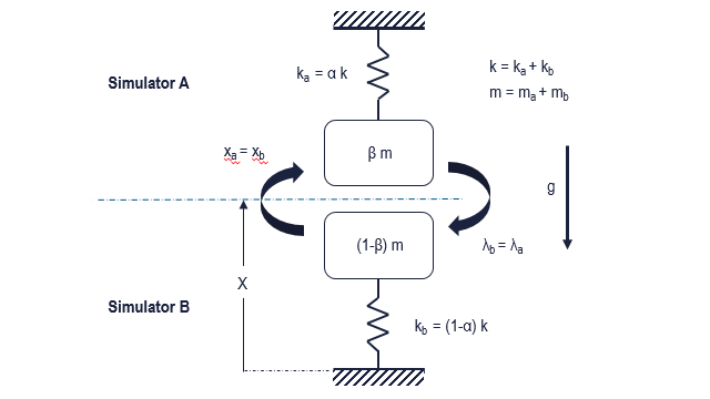
Figure 1. Dual mass spring systems.

Initially, both systems are at rest, and gravity is turned on at the start of the simulation such that the spring system oscillates. We define a constraint force, λ , between both systems to enforce that both masses move together. The system of equations:

m a x ¨ a + k a x a = − m a g − γ ,
m b x ¨ b + k b x b = − m b g − γ ,
with constraints and initial conditions:
x a = x b ,
x . a = x . b ,
x a = x b =   0.0         ⁢       a t ⁢               t = 0.0.

A stiffness distribution factor, α , defines the relative stiffness distribution between System A and System B compared to a total stiffness, k , for an equivalent single system:

k a = α k ,

k b = ( 1 − α ) k .

A mass distribution factor, β , defines the relative mass distribution between System A and System B compared to a total mass, m , for an equivalent single system:

m a = β m ,

m b = ( 1 − β ) m .

The radial frequency, ω , is defined as ω = k / m .

Simulator A receives the displacement, x b , from Simulator B and sets its displacement, x a . Simulator A then computes the acceleration, x ¨ a , and solves for the interface force, λ, according to

x ¨ a + α β ω 2 x a = − g − λ β m .

Simulator B receives the interface force, λ , from Simulator A and computes the acceleration according to

x ¨ b + ( 1 − α ) ( 1 − β ) ω 2 x b = − g − λ ( 1 − β ) m .

It then computes the velocity and displacement using Newmark’s time integration method. Its displacements, x b , are then exported to Simulator A.

Compiling the C++ Simulators

If you have not already done so, extract the SIMULIA Co-Simulation Services API kit as described in Extracting the SIMULIA Co-Simulation Services API Kit. The compiler needs access to the SIMULIA Co-Simulation Services header files, as discussed in Compiling your Application with SIMULIA Co-Simulation Services.

Typical compile options for compiling DualMassSpring_SystemA.cpp are as follows:

On Windows:

cl /c /W0 /MD /TP /I<location of CSS header files> DualMassSpring_SystemA.cpp

On Linux:

g++ -c -fPIC -w -Wno-deprecated /I <location of CSS header files> DualMassSpring_SystemA.cpp
Use similar options to compile DualMassSpring_SystemB.cpp.

Linking the Simulators

Depending on how you load the dynamic libraries, the linker might need access to the SIMULIA Co-Simulation Services dynamic libraries (see Linking the SIMULIA Co-Simulation Services to Your Application).

Typical link options for linking DualMassSpring_SystemA are as follows:

On Windows:

link /nologo /INCREMENTAL:NO /subsystem:console /machine:AMD64 /STACK:20000000 /NODEFAULTLIB:LIBC.LIB /DEFAULTLIB:kernel32.lib /DEFAULTLIB:user32.lib /DEFAULTLIB:advapi32.lib /FIXED:NO /LARGEADDRESSAWARE /out:.\DualMassSpring_SystemA.exe .\DualMassSpring_SystemA.obj /LIBPATH:<location of CSS .dll> ABQSMACseModules.lib msvcrt.lib

On Linux:

g++ -fPIC -Wl,-Bdynamic -Wl,--add-needed -o DualMassSpring_SystemA ./DualMassSpring_SystemA.o -L<path to CSS .so> -lABQSMACseModules
Use similar options to link DualMassSpring_SystemB.

Running the Coupled Simulation Using Two C++ Simulators

You run three processes for the coupled simulation:

  • The SIMULIA Co-Simulation Services Director;
  • Simulator A; and
  • Simulator B
We recommend that you run these processes in separate command shells, so that you can monitor each process during the development and debugging stages.

The SIMULIA Co-Simulation Services Director process and its command line arguments are described in SIMULIA Co-Simulation Services Director. You can start the SIMULIA Co-Simulation Services Director by either starting the SMACseCtlMain.exe function or by using the Abaqus execution procedure.

The Simulator command line arguments are as follows:

csedirector
Director in charge of the coupled simulation.

Specify the host:port where host is the host name or IP address of the machine from which the SIMULIA Co-Simulation Services Director is launched, and port is the listener port used by the SIMULIA Co-Simulation Services Director for this particular analysis.

alpha
Stiffness distribution factor.

This factor should be between 0.0 and 1.0.

beta
Mass distribution factor.

This factor should be between 0.0 and 1.0.

The commands below start the coupled simulation using the two simulator programs with the explicit Gauss-Seidel coupling scheme with the stiffness distribution factor set to 0.5 and the mass distribution factor set to 0.1. The SIMULIA Co-Simulation Services Director is launched on host earth with listener port 91000.

SMACseCtrlMain -config DualMassSpring_GaussSeidel_config.xml -listenerport 91000
SimulatorA -alpha 0.5 -beta 0.1 -csedirector earth:91000
SimulatorB -alpha 0.5 -beta 0.1 -csedirector earth:91000

The commands below start the dual mass-spring example using Simulator A and Abaqus with the implicit iterative coupling using Aitkens relaxation. The stiffness distribution factor is 0.5, and the mass distribution factor is 0.1. The SIMULIA Co-Simulation Services Director is launched using the Abaqus execution procedure on host mars with listener port 95000. The job name SimulatorB refers to the component instance name in the Co-Simulation Configuration file and differs from the input file name.

abaqus -cse -config DualMassSpring_Aitkens_Abaqus_config.xml -listenerport 95000
SimulatorA -alpha 0.5 -beta 0.1 -csedirector mars:95000
abaqus -job SimulatorB -input DualMassSpring_SystemB -csedirector mars:95000

Results

The solution of an equivalent single system is given by the differential equation:

x ¨ + ω 2 =   − g .
The closed form solution is
x ( t )   =   − g ω 2 ( 1 − cos ⁡ ( ω t ) ) ,
x ˙ =   − g ω sin ⁡ ( ω t ) ,
x ¨ =   − g ⁢     cos ⁡ ( ω t ) .

In this example, we have chosen a total stiffness equal to 35,000.0, a total mass equal to 2.5, a stiffness distribution factor of 0.5, and a mass distribution factor equal to 0.1. The closed-form solution for displacement, velocity, and acceleration is given above with a period of 0.0531.

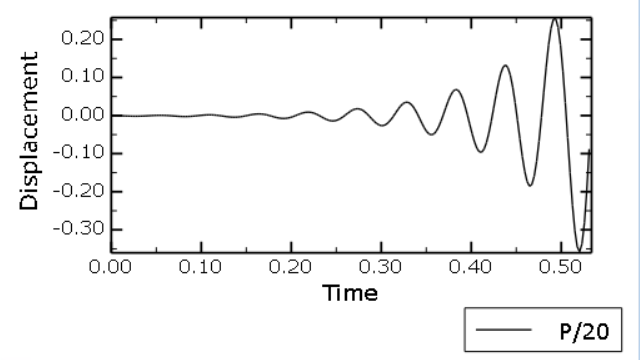
The simulation time is set to produce 10 cycles. A coupling step size equal to 1/20th of the period is selected. From a stability point of view, the coupled solution becomes unstable for explicit coupling, as shown in Figure 2 where an increase in amplitude is observed from cycle to cycle.

Figure 2. Displacement response using explicit coupling.

In some cases, selecting a smaller coupling step size might alleviate the stability issue. However, the solution cost increases and other numerical problems might arise with a smaller coupling step size. We recommend explicit coupling only for weakly coupled physics.

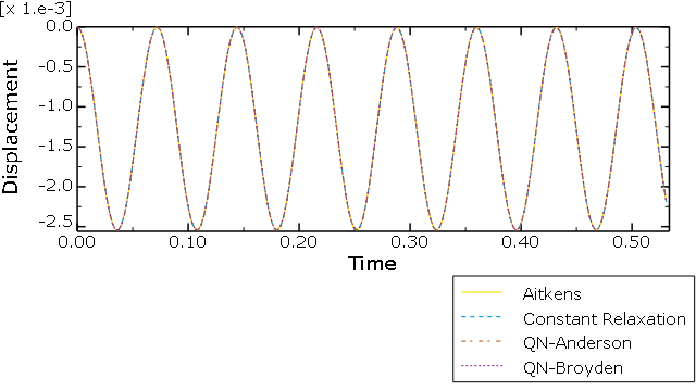
Figure 3 shows the displacement response for implicit iterative coupling using the constant relaxation, Aitken relaxation, Anderson quasi-Newton, and Broyden quasi-Newton accelerators.

Figure 3. Implicit coupling using accelerators for a coupling size of P/20.

The response is accurate and stable for the large coupling step size P/20. The constant relaxation method requires the most iterations to reach the specified convergence tolerance. In fact, after 30 iterations it was ended. The Aitken relaxation method takes on average 3 iterations, and the Anderson and Broyden quasi-Newton methods take an average of 4 iterations to converge. In more complex industrial problems, we expect the quasi-Newton methods to have fewer iterations than the Aitken relaxation method.

Files

The C++ code for the simulators, the Abaqus input file, and the configuration files are available in the examples/ folder in the SIMULIA Co-Simulation Services API kit (see SIMULIA Co-Simulation Services API Kit). If you have Abaqus installed, you can also use the abaqus fetch execution procedure.

DualMassSpring_SystemA.cpp
Code for spring-mass system A.
DualMassSpring_SystemB.cpp
Code for spring-mass system B.
DualMassSpring_SystemB.inp
Abaqus input file for System B.
DualMassSpring_GaussSeidel_config.xml
Configuration file using a Gauss-Seidel explicit coupling algorithm. Use this configuration file when coupling both simulators.
DualMassSpring_GaussSeidel_Abaqus_config.xml
Configuration file using Gauss-Seidel explicit coupling algorithm. Use this configuration file when coupling Simulator A with Abaqus.
DualMassSpring_ConstantRelaxation_config.xml
Configuration file using implicit iterative coupling with constant relaxation. Use this configuration file when coupling both simulators.
DualMassSpring_ConstantRelaxation_Abaqus_config.xml
Configuration file using implicit iterative coupling with constant relaxation. Use this configuration file when coupling Simulator A with Abaqus.
DualMassSpring_Aitkens_config.xml
Configuration file using implicit iterative coupling with Aitken relaxation. Use this configuration file when coupling both simulators.
DualMassSpring_Aitkens_Abaqus_config.xml
Configuration file using implicit iterative coupling with Aitken relaxation. Use this Configuration file when coupling Simulator A with Abaqus.
DualMassSpring_QNAnderson_config.xml
Configuration file using implicit iterative coupling and the quasi-Newton Anderson method. Use this configuration file when coupling both simulators.
DualMassSpring_QNAnderson_Abaqus_config.xml
Configuration file using implicit iterative coupling and the quasi-Newton Anderson method. Use this configuration file when coupling Simulator A with Abaqus.
DualMassSpring_QNBroyden_config.xml
Configuration file using implicit iterative coupling and the quasi-Newton Broyden method. Use this configuration file when coupling both simulators.
DualMassSpring_QNBroyden_Abaqus_config.xml
Configuration file using implicit iterative coupling and the quasi-Newton Broyden method. Use this configuration file when coupling Simulator A with Abaqus.