About Co-Simulation

The Abaqus co-simulation technique:

• can be used to solve complex fluid-structure interactions by coupling Abaqus with the SIMULIA Navier-Stokes solver (available in the Fluid Scenario Creation app on the 3DEXPERIENCE platform) or with a third-party CFD solver;

• can be used to solve problems involving electromagnetic-thermal or electromagnetic-mechanical interactions by coupling Abaqus with an electromagnetic analysis program, including electromagnetic analysis procedures in Abaqus/Standard, CST Studio Suite, or a third-party electromagnetic solver;

• can be used to solve general multiphysics simulations by coupling Abaqus with third-party and in-house analysis programs;

• can be used to solve complex multidomain analyses more effectively by coupling Abaqus/Standard to Abaqus/Explicit and Abaqus to Simpack;

• can be used for system-level modeling between logical and physical components; for example, coupling Abaqus with Dymola or any Functional Mockup Unit (FMU) using the FMI 2.0 standard;

• uses the SIMULIA Co-Simulation Engine to coordinate the coupled simulation;

• is intended for advanced users with in-depth knowledge of Abaqus, the other analysis program, and coupled solution methods;

• can be used with Abaqus models having linear or nonlinear structural response; and

• supports steady-state and transient procedures and time-harmonic procedures for electromagnetics.

The SIMULIA Co-Simulation Engine (CSE) consists of software components in charge of coordinating a coupled simulation, including sequential (see General Capability for Importing External Fields), submodeling (see Node-Based Submodeling), and co-simulation workflows. The SIMULIA Co-Simulation Engine consists of the following:

• software services (referred to as SIMULIA Co-Simulation Services) embedded into the clients (solver applications) and
• the SIMULIA Co-Simulation Engine Director in charge of controlling the coupled simulation.

The SIMULIA Co-Simulation Services (CSS) provide communication, algorithmic, mapping, transformation, and other services. Data between the clients, and control messages between the clients and the CSE Director, are communicated via the TCP/IP sockets. Conservative field mapping between interface regions having different mesh topologies is performed by the Field Mapper (see Field Mapper). The transformations services provide translation and rotation of source and target meshes, unit conversion, and field operations.

The CSE Director is a separate process that controls the exchanges between the clients in a coupled simulation. The Director process requires a CSE Configuration file, which specifies the configuration of the coupled multiphysics/multiscale problem. It specifies all the participants involved in the coupled simulation, the data exchange between each client, the coupling algorithmic, mapper specific settings, and more. The CSE Configuration File is an XML document that is usually generated by an authoring tool; typically, you do not need to create or modify it.

In a co-simulation the interaction between the numerical domains is through a common physical interface region over which data are exchanged in a synchronized manner between Abaqus and the coupled analysis programs. When coupling numerical domains to solve a multiphysics/multiscale problem, you must consider whether the numerical domains overlap or abut each other in order to define the domain coupling type. Domain coupling types include point coupling, surface coupling, and volume coupling (see Domain Coupling for Multiphysics and Multiscale Simulations).

One domain can affect the response of another domain through one or more of the following interactions:

• the constitutive behavior, such as the yield stress defined as a function of temperature or stress defined as a function of other solution fields, such as thermal strains or the piezoelectric effect;

• surface tractions/fluxes, such as a fluid exerting pressure on a structure;

• body forces/fluxes, such as Joule heating due to electrical current flow in a coupled thermal-electrical simulation;

• contact forces, such as the forces due to contact between a vehicle and an occupant/pedestrian modeled as separate domains;

• kinematics, such as fluid in contact with a compliant structure where the interface motion affects the fluid flow; and

• discrete coupling, such as sensor and actuation information.

You typically apply co-simulation techniques to problems where the most complex physics occurs within domains that are handled exclusively within an analysis. Due to the comparative numerical simplicity of the numerical techniques applied at the co-simulation interface, the physics controlling the interaction at the interface of the separate analysis domains (the strength of the physics coupling) might lead to stability and accuracy concerns.

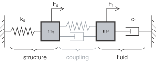
Figure 1 illustrates the coupling strength with an analogy in the frequency domain. Consider a lumped parameter dynamic system with a coupling impedance directly related to a response frequency $\omega$ . In a staggered solution approach each domain is solved by temporarily ignoring the coupling terms represented by the gray spring and dashpot in Figure 1.

Figure 1. Mechanical impedance analogy.

When the response frequency and coupling impedance are low, a staggered approach likely provides adequate solution accuracy and performance. However, when the response frequency is high (such that the coupling impedance is relatively large compared to the structure or fluid), you might encounter solution stability issues with the staggered approach.

Analysis domains are coupled in a staggered approach using either a globally explicit manner or an implicit iterative manner; that is, the equations for each domain are solved separately, and loads and boundary conditions are exchanged at the common interface. The SIMULIA Co-Simulation Engine supports different coupling schemes that can deliver robust and cost effective solutions to problems exhibiting different degrees of physics coupling strength.

In cases where the coupling is sufficiently weak, the coupling might be required only in one direction (such as when an electromagnetic force field contributes to the structural response, but a reverse coupling provides no significant impact on the electromagnetic field). A sequential solution approach is the most cost effective solution technique to solve these problems, although you can also run both solvers concurrently and exchange solution data in one direction only.

In an explicit staggered approach (such as the Gauss-Seidel coupling scheme), fields are exchanged only once per coupling step. This coupling strategy is applicable to problems that exhibit weak to moderate physics coupling (for example, aeroelasticity problems where you have air interacting with a relatively stiff structure). The explicit staggered approach is numerically cost effective, but it requires the use of a smaller coupling step size to obtain a stable and accurate solution.

In an implicit iterative approach, the fields are exchanged multiple times per coupling step until an overall equilibrium is achieved prior to advancing to the next coupling step. Implicit coupling is computationally more expensive per coupling step; however, in general, a larger coupling step size can be employed. Implicit schemes are appropriate for problems exhibiting moderate to strong physics coupling (for example, blood flow through an artery were the fluid density ratio between the fluid and solid is near unity, and the fluid is incompressible); however, this approach is limited to solvers that employ implicit time integration.

Accelerators can be employed with the implicit iterative approach to enhance the coupling by enlarging the convergence radius from a stability point of view. The SIMULIA Co-Simulation Engine supports two types of accelerator methods (relaxation technique and Quasi-Newton methods that approximate an inverse Jacobian at the interface) and can deliver close to an exact inverse Jacobian if sufficient past residual information is available.

The strength of the physics coupling can generally be greater when coupling two mechanical systems; for example, Abaqus/Standard to Abaqus/Explicit or Abaqus to Simpack. The SIMULIA Co-Simulation Engine supports coupling algorithms through communication of “right-hand-side” and “left-hand-side” terms to provide robust interface solutions across a wide range of problem parameters, which supports both implicit and explicit solvers.

For the latest support information and tips on running co-simulations with third-party analysis programs, see the Dassault Systèmes Knowledge Base at https://support.3ds.com/knowledge-base/.