Wind Turbine Tower–Frequency Analysis | ||
| ||
The FE Model
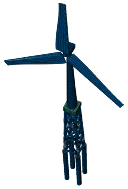
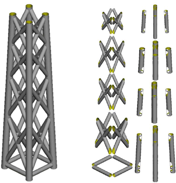
The model is for a modal analysis of a jacket structure that supports a 5MW offshore wind turbine. The structure is shown in Figure below, modeled with 3D shell elements. The remaining components of the wind turbine are modeled using continuum elements, membrane elements and rigid bodies, accounting for their correct inertial distribution. The foundations are represented by four piles that are fixed in the ground. Such wind turbines are subject to multiple periodic loads, such as wind loads and wave loads. Thus it becomes required to minimize the chances of a load frequency resonating with the natural frequency of the structure. The jacket structure is the core supporting structure for the turbine and is usually submerged fully or partially and becomes the loaded area. Thus it is a natural choice for optimization.
The requested discrete range is:
| Available Thicknesses | ||||
|---|---|---|---|---|
| 0.01 | 0.06 | 0.11 | 0.163 | 0.417 |
| 0.015 | 0.065 | 0.115 | 0.17 | 0.455 |
| 0.02 | 0.07 | 0.12 | 0.191 | 0.531 |
| 0.025 | 0.075 | 0.125 | 0.208 | 0.607 |
| 0.03 | 0.08 | 0.13 | 0.229 | 0.683 |
| 0.035 | 0.085 | 0.135 | 0.246 | 0.759 |
| 0.04 | 0.09 | 0.14 | 0.267 | 0.836 |
| 0.045 | 0.095 | 0.145 | 0.305 | 0.912 |
| 0.05 | 0.1 | 0.15 | 0.343 | 1 |
| 0.055 | 0.105 | 0.152 | 0.378 | |
| The FE model of the entire wind turbine |
|---|
 |
| Break down of the jacket structure |
|---|
 |
Optimization Problem
The Jacket structure is chosen as the optimization domain. The eigenfrequencies of this structure are maximized, while keeping the volume constant. It is preferable to have constant volume, so that the buoyancy calculations do not must be redone and the overall stability of the structure is not affected. The thicknesses of the tubes in the jacket are the design variables; most importantly, the result from the optimization should be manufacturable. This means the following:
- Each tube unit should have a uniform size.
- The sizes should be from standard sizes or at least manufacturable (for example 0.015 cm thickness is good, but 0.015733 cm is not).
  . . .

  DVCON_SIZING
   ID_NAME        = MY_DVCON_SIZING_BOUNDS
   CHECK_TYPE     = THICKNESS_BOUNDS
   EL_GROUP       = S_OPT_GROUP
   LOWER_BOUND    = 0.0002
   UPPER_BOUND    = 1.0
   MAGNITUDE      = ABS
  END_

  . . .

  DVCON_SIZING
   ID_NAME         = DVCON_SIZING_set_discr
   EL_GROUP        = ALL_ELEMENTS
   CHECK_TYPE      = DISCRETE
   DISCR_LIST_FILE = Sheet_sizing_turbine.csv
   DISCR_CYCLE     = 9
   DISCR_INTERVAL  = 4
   DISCR_FRACTION  = 0.2
   DISCR_CHANGE    = 10
  END_

  . . .

  OPT_PARAM
    STOP_CRITERION_ITER= 28
  END_

  . . .
Optimization Results
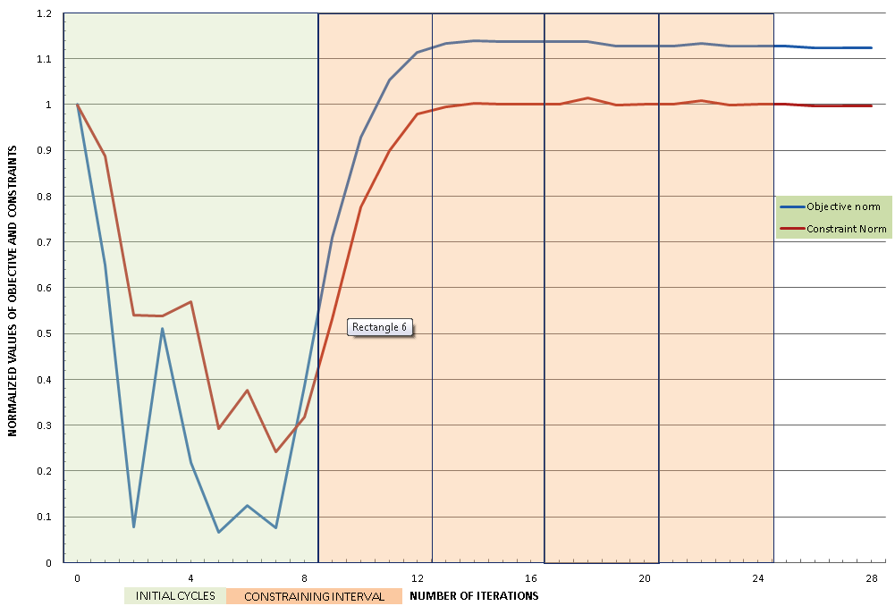
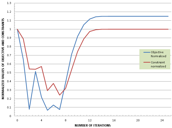
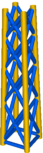
The figures below show the result and a comparison between the optimization with continuous and discrete variables.
| History of objective and constraints from the sizing optimization for discrete variables. |
|---|
 |
| History of objective and constraints from the sizing optimization for continuous variables. |
|---|
 |
| Resulting thicknesses of the sizing optimization for discrete variables. | |
|---|---|
 |
 |
Resulting thicknesses of the sizing optimization for continuous variables. | |
|---|---|
 |
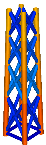 |
The difference in the objective functions for the standard and discrete optimization is less than 2% and the constraints are fulfilled within an error of 0.001 in this example.