Frequency Spectrum

Limitations

Currently frequency responses are allowed only for sizing optimization.

Overview

Frequency response is obtained using ANTYPE, 3 or ANTYPE,SPECTR in the CDB finite element input file. The different solution methods for calculating the spectrum in ANSYS® are activated using HROPT. The three following methods are supported in Tosca Structure:

HROPT,FULL
This is the full solution method.
HROPT,REDUC
- Reduced solution method (deals only with main nodes, can be viewed as an extension of the Mode Superposition Method)
- By default, the reduced solution method writes the reduced results to the RFRQ file. However, the reduced results must be expanded to the entire results in the RST file. Therefore, the following has to be added in the CDB finite element input file:
  - EXPASS,ON for obtaining the response for all nodes.
  - NUMEXP for defining the frequency range to be expanded.
  - HROUT, ON, OFF, for printing the real and imaginary components (ON is also default) and for uniform spacing of the excitation frequencies (OFF is also default). HROUT, ON, ON for eigenvalue-dependent spacing is also allowed.

HROPT,MSUP

Superposition, the most used option for large models because it is very fast. However, it is requiring that the eigenfrequencies (ANTYPE, 2 and the number of eigenfrequencies) are initially calculated.

Important:

This method can give quite wrong results for low-excitation frequencies corresponding to the almost static load case:

EXPASS,ON for obtaining the response for all nodes.
NUMEXP for defining the frequency range to be expanded.
HROUT, ON, OFF, for printing the real and imaginary components (ON is also default) and for uniform spacing of the excitation frequencies (OFF is also default). HROUT, ON, ON for eigenvalue-dependent spacing is also allowed.

Direct Solution

In the following, an example of a part of a load case file (file.s*) using the solution method HROPT,FULL is shown:


.........
ANTYPE, 3 ! frequency response
ALPHAD, 0.01 ! Viscous mass damping
BETAD, 0.02 ! Viscous stiffness damping
DMPRAT, 0.03 ! Structural stiffness damping
HROPT,FULL ! Direct solution method
HROUT,ON,OFF ! Uniform spacing (default)
NSUBST, 405 ! Number of substeps
HARFRQ,0,500 ! Frequency range
OUTPR,ALL,NONE ! No output in ASCII format
.........

Below an example of a part of a CDB file using load cases based on

HROPT,FULL

is shown:


................
/GO
FINISH
! ---------------------------------------------------
/SOLU
HROUT,ON,OFF ! Both real and imaginary part
OUTPR,ALL,NONE ! No output in ASCII format
LSSOLVE,1,1,12 ! In this case 12 load cases
FINISH
................

Modal Decomposition

In the following, an example of a part of a load case file (file.s*) using the solution method HROPT,MSUP (or HROPT,REDUC) is shown:

.........
ANTYPE, 3 ! frequency response
ALPHAD, 0.01 ! Viscous mass damping
BETAD, 0.02 ! Viscous stiffness damping
DMPRAT, 0.03 ! Structural stiffness damping
HROPT,MSUP,25,1 ! Mode superposition method
HROUT,ON,OFF ! Uniform spacing (default)
NSUBST, 405 ! Number of substeps
HARFRQ,0,500 ! Frequency range
OUTPR,ALL,NONE ! No output in ASCII format
.........

An example of a part of a CDB file using load cases based on HROPT,REDUC or HROPT,MSUP is shown below.

Note:

The CDB file should have the name model.cdb in this example. If another file name for the CDB file is applied, then the file name "model" should be substituted with the other file name.

In the given example, the frequency range is going from 0 Hz to 500 Hz using 105 increments. The user can also apply NUMEXP,ALL.


..........
/GO
FINISH
! ---------------------------------------------------
! Modal (Eigenfrequency) solution
/SOLU
LSSOLVE,1,1,1
/COPY,file,rst,,model_1,rst
FINISH
! ---------------------------------------------------
! Frequency response solution
! ---------------------------------------------------
! Load case 2: Frequency response 1
! use the results of the modal analysis
/SOLU
/COPY,model_1,rst,,file,rst
LSSOLVE,2,2,1
FINISH
! expansion of the solution
/SOLU
/assign,rst,model_2,rst
EXPASS,ON
OUTPR,ALL,NONE ! No output in ASCII format
NUMEXP, 105, 0.0, 500.0 ! the frequency range to expand
HROUT,ON,OFF ! both real and imaginary part
SOLVE
FINISH
! ---------------------------------------------------
! Load case 3: Frequency response loadcase 2
! use the results of the modal analysis
/SOLU
/COPY,model_1,rst,,file,rst
LSSOLVE,3,3,1
FINISH
! expansion of the solution
/SOLU
/assign,rst,model_3,rst
EXPASS,ON
OUTPR,ALL,NONE ! No output in ASCII format
NUMEXP, 105, 0.0, 500.0 ! the frequency range to expand
HROUT,ON,OFF ! both real and imaginary part
SOLVE
FINISH
! ---------------------------------------------------
! Load case 4: Frequency response loadcase 3
! use the results of the modal analysis
/SOLU
/COPY,model_1,rst,,file,rst
LSSOLVE,4,4,1
FINISH
! expansion of the solution
/SOLU
/assign,rst,model_4,rst
EXPASS,ON
OUTPR,ALL,NONE ! No output in ASCII format
NUMEXP, 105, 0.0, 500.0 ! the frequency range to expand
HROUT,ON,OFF ! both real and imaginary part
SOLVE
FINISH
..............

Important:

Significant improvement in the CPU-time is obtained using the following command in each load case. This ensures that no ASCII information is written as output. Therefore, adding this command in each load case is strongly recommended.:
```
OUTPR,ALL,NONE ! No output in ASCII format
```
Significant improvement in the CPU-time is obtained using the following command in each load case. This ensures that only nodal results are written to the database. Therefore, adding these commands in each load case is strongly recommended:
```
OUTRES,ALL,NONE ! No output in binary format (rst-file)
OUTRES,NSOL,ALL ! Output only node results (displacements)
```
Prescribed displacements and thereby indirectly velocities, and accelerations for ANSYS® are supported in frequency response using the command D for defining degree of freedom constraints at nodes. Other types of prescribed displacements, velocities, and accelerations for ANSYS® are not supported.

General Damping Matrices in ANSYS®

The general damping matrix [C] of the structure can be written as


$[C] = α [M] + (β + β_{c}) [K] + \sum_{j = 1}^{N_{m}} [(β_{j}^{m} + \frac{2}{Ω} β_{j}^{ξ}) [K_{j}]] + \sum_{k = 1}^{N_{e}} [C_{k}] + [C_{ξ}]$

with


$[K]$ =	structural stiffness matrix
$[M]$ =	structural mass matrix
$Ω$ =	circular excitation frequency
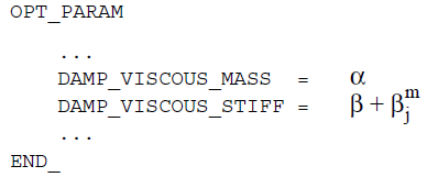
$α$ =	mass matrix multiplier for viscous damping (input in ANSYS® using the ALPHAD command)
$β$ =	stiffness matrix multiplier for viscous damping (input in ANSYS® using the BETAD command)
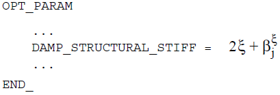
$β_{c}$ =	variable stiffness matrix multiplier for structural damping $β_{c} = (2 / Ω) ξ$ Important note: for modal superposition is DMPRAT modal damping and therefore NOT allowed.
$β_{j}^{m}$ =	stiffness matrix multiplier for material j for viscous damping (input as a material property using the DAMP label on the MP command)
$N_{m}$ =	is the number of materials with DAMP Note: this number should include all elements in the design domain and in the manufacturing constraints.
$β_{j}^{ξ}$ =	stiffness matrix coefficient for material j for structural damping (input as DMPR on MP command)
$C_{k}$ =	element damping matrices in general form (are always permissible)
$C_{ξ}$ =	eigenfrequency dependent damping matrix Note: not supported, damping defined through MDAMP is prohibited

Allowable viscous damping for design elements in ANSYS®:

Allowable structural damping for design elements in ANSYS®: