Remarks for Sensitivity-Based Optimizations

Using Design Response Values and Sensitivities Calculated by Abaqus

In the context of topology, sizing, shape, and bead optimization, design response values, and the corresponding sensitivities can be calculated directly by the Abaqus solver. This option is activated automatically by the optimization system in cases where it is applicable. It is possible to change this behavior by setting the following option, but it is not recommended:

OPTIONS
 SENS_CALC_MODE = AUTOMATIC (Default) | SOLVER | TOSCA | HYBRID
END_

If the above option is set to TOSCA, the design response values and the corresponding sensitivities will be calculated by the optimization system. Setting this option to SOLVER enforces the system to use solver sensitivities and design response values. If HYBRID is chosen, the design response values and the corresponding sensitivities will be calculated by the solver if they are supported and by the optimization system for all other cases. Setting this option to AUTOMATIC lets the optimization system choose the right mode for calculating the design response and sensitivity values. To be able to use older versions of Abaqus (older than 3DEXPERIENCE2017x FP1721), set SENS_CALC_MODE = TOSCA.

Traditionally, the solver is called in each optimization iteration and is given the modified input file to calculate the necessary results for the optimization system. Each time the licenses are checked out, the preprocessor is run, a finite element analysis is performed, the results are written to the database, and the solver is shut down. This means that there is a sequence of solver calls. Alternatively, for topology optimization, it is possible to call the solver just once at the beginning of the optimization procedure, and instead of shutting it down each iteration, a number of distribution tables are updated when the design is changed and then the solver is closed at the end of the optimization procedure. This means that for all the optimization iterations the same (simultaneous) solver session is used. Running the solver in simultaneous mode can increase the run time performance. The solver run mode is chosen automatically by the optimization system. This behavior can be changed by setting the following option, but it is not recommended:

OPTIONS
 SOLVER_RUN_MODE = AUTOMATIC (Default) | SEQUENTIAL | SIMULTANEOUS
END_

The advantages for topology, sizing, shape, and bead optimization using solver design response values and the corresponding sensitivities are:

• For stress design responses in topology optimization (TYPE = SIG_TOPO_MISES or its equivalent TYPE = SIG_SENS_MISES ), all structural element types are supported.
• Material, geometric, and contact nonlinearities are supported.
• Stress design responses for sizing are available (TYPE=SIG_SIZING_MISES or its equivalent TYPE=SIG_SENS_MISES ).
• For reaction and internal force design responses, all coupling types (for example, *mpc, *equation and *kinematic in *coupling ) and all element types are supported.
• All prescribed acceleration types are supported.
• Magnitude-design responses are supported for 2D models.
• The addition of a primal solution from the general step to the primal solution of the following step perturbation (with or without load case) for the design responses is supported.
• The LCP solver for efficient optimization of small-sliding frictionless contact models is supported.
• The option fixed in command *boundary is supported.
• For *plasticity materials, better accuracy in sensitivity analysis can be achieved.
• Distributed load type label CENT (centrifugal loads) is supported.
• Distributed load type label CORIO (Coriolis force loading) is supported.
• Distributed load type label GRAV (gravity loading) is supported for shape optimization.
• To define operator design responses (TYPE = OPER), responses of SINGLE nodes from different load cases can be used.

The current limitations are:

• Mode tracking can be performed only when the number of eigenfrequencies calculated by the solver is not changing between the optimization iterations. The number of requested eigenfrequencies should be specified by the user in the solver input file. The request of the eigenfrequencies range is not supported.
• If the *model change command is used in the solver input file, you should set the option ABQ_SENS_ABSENT_SET_ZERO=YES.
• Currently quantities on secondary nodes of MPCs cannot be used to define design responses. The corresponding sensitivity will be just zero.
• In the context of topology optimization, using solver design response values and the corresponding sensitivities and activating the SOFT_DELETE option the deleted elements are not removed from the modified solver input file. Their stiffness and mass scaling factors are just set to zero in the corresponding distribution tables. The mass and stiffness contributions of these elements are neglected by the solver.

The differences for topology optimization are:

• Von Mises stress constraints and the corresponding sensitivities are calculated taking the following relation into account:

  $\underset{elem}{Max}\left|\frac{{\sigma }_{von}}{f\left({\rho }_i\right)}\right|\le {\sigma }_{ref}$

  The reference stress value on the right side of this equation is the constraint value. On the left side, the von Mises stress is scaled by some interpolation function depending on the current values of pseudo density.
• Von Mises stress terms in objective function and the corresponding sensitivities are calculated taking the following relation into account:

  $OBJ={\alpha }_1\underset{elem}{Max}\left|\frac{{\sigma }_{{von,}_1}}{f\left({\rho }_i\right){\sigma }_{{ref,}_1}}\right|+{\alpha }_2\underset{elem}{Max}\left|\frac{{\sigma }_{{von,}_2}}{f\left({\rho }_i\right){\sigma }_{{ref,}_2}}\right|+\mathrm{...}={\alpha }_1\frac{{DRESP}_1}{{\sigma }_{{ref,}_1}}+{\alpha }_2\frac{{DRESP}_2}{{\sigma }_{{ref,}_2}}+\mathrm{...}$

  In cases where the user is not giving reference values for stress objective terms, the initial design response values (from iteration zero) are used:

  $OBJ={\alpha }_1\frac{{DRESP}_1}{{DRESP}_{1,iter=0}}+{\alpha }_2\frac{{DRESP}_2}{{DRESP}_{2,iter=0}}+\mathrm{...}$

  It is always recommended that you provide reference for the stress objective terms. Otherwise, the objective values reported by Tosca will be difficult to interpret or will be not interpretable at all.

Prescribed Accelerations for Sensitivity-Based Optimization Using Tosca Response Values and Sensitivities

Prescribed acceleration loading is often caused by gravity fields, centrifugal loading, and rotary acceleration loads. This chapter defines which kinds of acceleration types for the Abaqus solvers are feasible for sensitivity-based topology and sizing optimization. These acceleration types are not supported for shape and bead optimization.

The following commands are supported for acceleration loading:

• GRAV: Gravity loading.
• CENTRIF: Centrifugal load
• ROTA: Rotary acceleration load

The following are not supported:

• CENT: Centrifugal load is not supported.
• CORIO: Coriolis force loading is not supported.

Several CPU-Processors in Combination with Sensitivity-Based Topology Optimization

This option is relevant only for SENS_CALC_MODE = TOSCA and is not necessary using default settings for Abaqus.

Abaqus fails to deliver all results requested by Tosca Structure sensitivity-based topology optimization when an Abaqus analysis is executed using more than one CPU-processor in combination with Tosca Structure sensitivity-based topology optimization. Abaqus failing to deliver all results requested by Tosca Structure sensitivity-based topology optimization is solved by adding the following in the OPT_PARAM command,

OPT_PARAM
  ....
  PROCESSORS = MULTI
  ....
END_

Temperature Loading

The following commands are supported for temperature loading exclusively in sensitivity-based topology optimization: *TEMPERATURE.

Cyclic Symmetry Model

The *CYCLIC SYMMETRY MODEL command is not supported in sensitivity-based topology and sizing optimization using sensitivities calculated by Tosca. Using sensitivities calculated by Abaqus, this limitation is avoided.

Showing Consistent Values for Stress and PEMAG Design Responses

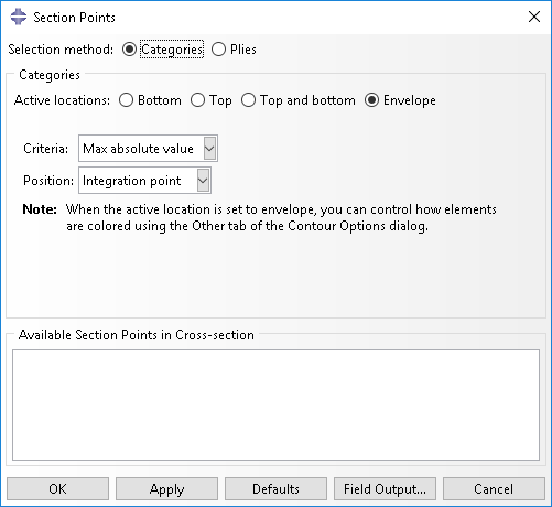
For consistency with Tosca / Abaqus values, use max absolute values at integration points and no averaging in Abaqus/CAE since the integration points are used for the evaluations. This can be done by selecting Result > Result Options and Result > Section Points from the main menu bar, respectively. Refer to the figures below for more details.

Group Operator Evaluation with Abaqus

Tosca Structure now provides the capability to use large groups of more than 5000 elements or nodes in the design response definition in an efficient way. This is done by using a new algorithm in Abaqus to evaluate the value using the OPERATOR entry in the *DESIGN RESPONSE option. To activate this feature, use the following OPTIONS command:

OPTIONS
 DRESP_GROUP_OPER_AGGREGATION = OFF (Default) | ON 
END_

The group operator types MAX, MIN, SUM, and AVERAGE will be supported. In the case of a MAX/MIN group operator in a design response, Abaqus and Tosca Structure evaluate these in different ways as explained below.

Classically, a MAX/MIN group operator is nondifferentiable and thus an approximation must be used to calculate sensitivities. The new evaluation method in Abaqus uses an aggregation method that creates a differentiable operator that delivers a value closer to the actual MAX/MIN

Inertia Relief

Inertia relief is often used in aerospace and automotive analyses, the latter often in combination with Multi-Body Dynamics like Simpack. This is a simulation feature where the inertia of the component is used to create static equilibrium. It is specified in the input file:

*INERTIA RELIEF