Material Interpolation

Recall that the original topology optimization problem is formulated as an integer problem (see, for example, Bendsøe and Sigmund [2003])


$p_{e} = 1$ or $p_{e} \approx 0$

meaning that each element should be filled up with material (solid elements with the relative material volume equal to 1) or contain no material (void elements with the relative material volume close to 0, but always positive). Thus, the relative material volume of each element is defined as a design variable. Numerically, the above optimization problem is an integer problem and difficult to solve for a large number of design variables. Therefore, the above optimization problem is relaxed so the relative densities can have values in between 0 and 1,


$p_{e} =] 0, 1]$ .

The material interpolation schemes penalizing the Young’s modulus E for the intermediate densities are introduced for obtaining the solution of the relaxed problem resulting in all elements being either solid or void elements. Tosca Structure contains multiple material interpolation schemes described in the following.

SIMP Interpolation

The SIMP (Solid Isotropic Material with Penalization) material interpolation scheme is defined by


$E = E_{0} ρ^{p}$

and is very popular in the literature; see, for example, Mlejnek (1992), Bendsøe and Sigmund (1999), and Bendsøe and Sigmund (2003) and references therein. The Young’s modulus $E_{0}$ is the Young’s modulus when the element is fully solid material, thus being the Young’s modulus defined by the user. The penalty factor p defines to what extent the solution is forced toward a solution with solid or void elements only. The penalty factor p should be greater than 1. Numerical experiments indicate that p=3 is a good value.

RAMP Interpolation

The RAMP (Rational Approximation of Material Properties) material interpolation scheme is defined by


$E = E_{0} \frac{ρ}{1 + p (1 - ρ)}$

The RAMP interpolation scheme is desirable for dynamic problems because the interpolation scheme is concave, see Hansen (2005) and Stolpe and Svanberg (2001). For the RAMP interpolation scheme, the interpolation factor p should be greater than 0. Numerical experiments indicate that p=3 is a good value.

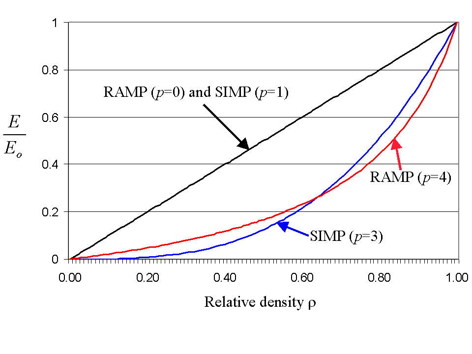
The following figure shows the interpolation of the Young’s modulus for the SIMP and RAMP material scheme, respectively.

For p=1 in SIMP and p=0 in RAMP, the material interpolation is the so-called thickness optimization problem that leads to many elements having intermediate densities. By increasing the penalization factor p, the intermediate densities turn out to be computationally more expensive because elements having intermediate densities require a higher density for having the same stiffness as in the thickness optimization problem. Thus, when the penalty factor is increased, fewer elements have an intermediate density. However, one should not choose a too large penalty factor because then the likelihood for ending up in a local minimum during the optimization is significantly higher. If the penalty factor is extremely high, you will always end up in a local minimum.

Consequently, a compromise for the penalty factor will be to choose a value in the interval between 2 and 4 that also agrees with the numerical experiments.

PEDE Interpolation

By default, the optimization algorithm chooses the SIMP interpolation scheme with p=3. However, if at least one dynamic load case is used or body loads are present in the model (for example, gravity), the interpolation scheme is switched to PEDE automatically.

Tosca Structure might generate different results if the optimization setup is changed in such a way that would lead to a switch of the interpolation scheme. This can happen even if one would not expect an influence of the change (for example, adding a nonactive frequency constraint or changing to an otherwise identical gravity loading). Setting the interpolation scheme in the optimization parameters will prevent the automatic switch.

The PEDE interpolation might lead to convergence problems if stresses play a role in the optimization. It is highly recommended to use MIMP interpolation in this case.

The PEDE material interpolation scheme is proprietary. Therefore, further details are omitted here.

MIMP Interpolation

The MIMP material interpolation is a combination of the SIMP for the constitutive material interpolation and a new material interpolation for the physical density. It is recommended for strength optimizations where the stress is applied in either objective or constraint, especially when mass-dependent quantities (for example, acceleration forces) are present. It also improves optimization results for setups with inactive, mass-related design responses, such as frequency, where Tosca Structure would change per default the material interpolation to PEDE.

In contrast to the other interpolation schemes, when the MIMP interpolation is used, Tosca Structure applies the design variable filter algorithm instead of the sensitivities filter.

The MIMP material interpolation scheme is proprietary. Therefore, further details are omitted here.

4th-Order Interpolation

The 4_TH (4th-order polynomial) material interpolation is defined by


$E = E_{0} (a_{4} ρ^{4} + a_{3} ρ^{3} + a_{2} ρ^{2} + a_{1} ρ + α_{0})$

This interpolation scheme should be used only by experienced users. The coefficients must be defined in a way that the material interpolation is positive in the given range of the relative density. It is up to the user that physical bounds are fulfilled; for example, the Hashin-Shtrikman bounds. By default, there is no penalization built in, meaning that one would not yield solid-void designs.

Command Examples

The user has the possibility to choose the interpolation scheme and the value of the penalty factor using the commands MAT_INTERPOLATION and MAT_PENALTY, respectively. The valid values for MAT_INTERPOLATION parameter are SIMP, RAMP, PEDE, MIMP and 4_TH.

For example, the SIMP material interpolation scheme and a penalty of 3.5 are used in the following example:

OPT_PARAM
 ID_NAME           = opt_params
 OPTIMIZE          = id_of_optimize
 ...
 MAT_INTERPOLATION = SIMP
 MAT_PENALTY       = 3.5
END_

The RAMP material interpolation scheme and a penalty of 2.5 are used in the following example:

OPT_PARAM
 ID_NAME           = opt_params
 OPTIMIZE          = id_of_optimize
 ...               
 MAT_INTERPOLATION = RAMP
 MAT_PENALTY       = 2.5
END_

The 4_TH material interpolation scheme and the corresponding coefficients are defined in OPT_PARAM command as follows:

OPT_PARAM
 ID_NAME           = opt_params
 OPTIMIZE          = id_of_optimize
 ...
 MAT_INTERPOLATION = 4_TH
 MAT_0_TH_FACTOR   = 0.0
 MAT_1_TH_FACTOR   = 0.0
 MAT_2_TH_FACTOR   = 0.0
 MAT_3_TH_FACTOR   = 3.0
 MAT_4_TH_FACTOR   = 0.0
END_

For the 4_TH material interpolation scheme, the user should also set the required lower and upper bounds for the relative density using, for example, the following commands:

OPT_PARAM
 ...
 DENSITY_LOWER     = 0.4
 DENSITY_UPPER     = 0.9
 ...
END_